On September 16, Arctic sea ice likely reached its annual minimum extent of 4.72 million square kilometers (1.82 million square miles). The 2021 minimum is the twelfth lowest in the nearly 43-year satellite record. The last 15 years are the lowest 15 sea ice extents in the satellite record. The amount of multi-year ice (ice that has survived at least one summer melt season), is one of the lowest levels in the ice age record, which began in 1984.

In the Antarctic, sea ice extent is now falling rapidly, but it is still too early to assume that the maximum has been reached. The maximum for Antarctic sea ice typically occurs in late September or early October. However, Antarctic sea ice extent is highly variable near the maximum because of storms acting to expand or compact the extended ice edge.

Please note that this is a preliminary announcement. Changing winds or late-season melt could still reduce the Arctic ice extent, as happened in 2005 and 2010. NSIDC scientists will release a full analysis of the Arctic melt season, and discuss the Antarctic winter sea ice growth, in early October.

Overview of conditions

Figure 1. Arctic sea ice extent for September 16, 2021, was 4.72 million square kilometers (1.82 million square miles). The orange line shows the 1981 to 2010 average extent for that day. Sea Ice Index data. About the data

Credit: National Snow and Ice Data Center
High-resolution image

On September 16, sea ice reached its annual minimum extent of 4.72 million square kilometers (1.82 million square miles) (Figure 1). In response to the setting sun and falling temperatures, ice extent has begun rising and will continue to rise through autumn and winter. However, a shift in wind patterns or a period of late season melt could still push the ice extent lower.

The minimum extent was reached two days later than the 1981 to 2010 median minimum date of September 14. The interquartile range of minimum dates is September 11 to September 19.

Conditions in context

Figure 2. The graph above shows Arctic sea ice extent on September 16, 2021, along with several other recent years and the record minimum set in 2012. 2021 is shown in blue, 2020 in green, 2019 in orange, 2018 in brown, 2017 in magenta, and 2012 in dashed brown. The 1981 to 2010 median is in dark gray. The gray areas around the median line show the interquartile and interdecile ranges of the data. Sea Ice Index data.

Credit: National Snow and Ice Data Center
High-resolution image

This year’s minimum set on September 16 was 1.33 million square kilometers (514,000 square miles) above the record minimum extent in the satellite era, which occurred on September 17, 2012 (Figure 2). It is also 1.50 million square kilometers (579,000 square miles) below the 1981 to 2010 average minimum extent, which is equivalent to twice the size of Texas.

In the 43-year-satellite record, 15 of the lowest minimums have all occurred in the last 15 years.

Multiyear ice extent is one of the lowest on record. First-year-ice coverage increased dramatically since last year, jumping from 1.58 million square kilometers (610,000 square miles) to 2.71 million square kilometers (1.05 million square miles). The increase in total extent from last year’s minimum to this year’s is hence comprised of first-year ice.

The overall, downward trend in the minimum extent from 1979 to 2021 is 13.0 percent per decade relative to the 1981 to 2010 average. The loss of sea ice is about 80,600 square kilometers (31,100 square miles) per year, equivalent to losing the size of the state of South Carolina or the country of Austria annually.

Fifteen lowest minimum Arctic sea ice extents (satellite record, 1979 to present)

Values within 40,000 square kilometers (15,000 square miles) are considered tied. The 2020 value has changed from 3.74 to 3.82 million square kilometers (1.47 million square miles) when final analysis data updated near-real-time data. The 2020 date of minimum also changed from September 15 to September 16. 

The Arctic sea ice minimum extent is imminent. After a cool and stormy summer, this year’s minimum extent will be one of the highest of the past decade, despite the amount of multiyear ice standing at a near-record low. A large area of low ice concentration persists in the Beaufort and Chukchi Seas, and some of this may still be compacted by winds or melt away because of the remaining heat in the upper ocean.

Overview of Conditions

Figure 1a. Arctic sea ice extent for September 15, 2021 was 4.73 million square kilometers (1.83 million square miles). The orange line shows the 1981 to 2010 average extent for that day. Sea Ice Index data. About the data

Credit: National Snow and Ice Data Center
High-resolution image

Figure 1b. This map shows Arctic sea ice concentration based on data from the Advanced Microwave Scanning Radiometer 2 (AMSR2) data as of September 14, 2021. Yellows indicate sea ice concentration of 75 percent; dark purples indicate sea ice concentration of 100 percent.

Credit: University of Bremen
High-resolution image

As of September 15, Arctic sea ice extent stood at 4.73 million square kilometers (1.83 million square miles), placing it tenth lowest in the satellite record for the date. While extent continues to decline as of this post, the seasonal minimum is likely to occur soon, depending on how much heat remains in the upper ocean and on winds, which can compact the ice cover or spread it out. If the winds push the ice poleward, this may further reduce the total extent. Nevertheless, the seasonal minimum extent promises to be one of the highest of the past decade—only 2013, 2014, and 2018 are currently tracking above the 2021 sea ice extent.

It has been an odd summer. While fairly cool and stormy summer conditions limited summer melt, as discussed in our earlier post, the amount of multiyear ice is at a record low, roughly one-fourth of the amount seen in the early 1980s. Ice loss the first two weeks of September primarily occurred in the Beaufort and Chukchi Seas, and to a lesser extent also surrounding Severnaya Zemlya. As seen in Advanced Microwave Scanning Radiometer 2 (AMSR-2) imagery (Figure 1b), areas of low concentration ice persist in the Beaufort and Chukchi Seas; how much of this ice melts away largely depends on ocean heat. Satellite mapping of sea surface temperatures shows much of the open ocean surrounding the low ice concentration area is already near the freezing point. By contrast, the compact, well-defined ice edge along most of the Russian side of the Arctic Ocean indicates that freezing is already underway in this area.

Conditions in context

Figure 2a. This plot shows the departure from average air temperature in the Arctic at the 925 hPa level, in degrees Celsius, between September 1 to 13, 2021. Yellows and reds indicate higher than average temperatures; blues and purples indicate lower than average temperatures.

Credit: NSIDC courtesy NOAA Earth System Research Laboratory Physical Sciences Laboratory
High-resolution image

Figure 2b. This plot shows average sea level pressure in the Arctic in millibars from September 1 to 13, 2021. Yellows and reds indicate high air pressure; blues and purples indicate low pressure.

Credit: NSIDC courtesy NOAA Earth System Research Laboratory Physical Sciences Laboratory
High-resolution image

Air temperatures at the 925 hPa level (about 2,500 feet above the surface) as assessed over the first 13 days of September were near average over most of the Arctic Ocean. Temperatures from 2 to 4 degrees Celsius (4 to 7 degrees Fahrenheit) above average were the rule along the coasts of the Kara and Laptev Seas (Figure 2a). In sharp contrast to the persistent pattern of low pressure over the Arctic Ocean characterizing this summer, the first 13 days of September saw high average air pressure (Figure 2b).

Focus on the Northwest Passage

Figure 3. These graphs show the total sea ice area along each Northwest Passage route (y axis) by day (x axis) dating back to 1981. The top graph shows the northern route and the bottom graph shows the southern route. 

Credit: Canadian Ice Service
High-resolution image

Data from the Canadian Ice Service compiled by colleague Steve Howell of Environment and Climate Change Canada allows for a closer look at sea ice conditions in the Northwest Passage. While there are multiple Northwest Passage routes, most attention is focused on the southern route, known as Amundsen’s route, entered from the Pacific side through Amundsen Gulf, and the northern route entered from the Pacific side via M’Clure Strait. This wide, deeper-water route is the one that might become a viable waterway for commercial shipping in the future. As of early to mid-September, the northern deep-water route is choked with ice and will not open this year; ice conditions are quite severe compared to the past couple of decades. By contrast, there is much less ice in the southern route, approximately 30,000 square kilometers (11,600 square miles). Most of this is located on Somerset and Prince of Wales Islands. On the other side of the Arctic, the Northern Sea Route is essentially open, though some areas of ice remain near Severnaya Zemlya.

Antarctic oddities

Figure 4. Antarctic sea ice extent for September 15, 2021 was 18.64 million square kilometers (7.20 million square miles). The orange line shows the 1981 to 2010 average extent for that day. Sea Ice Index data. About the data

Credit: National Snow and Ice Data Center
High-resolution image

Antarctic sea ice extent is approaching its seasonal maximum, which typically occurs in late September. A surge in sea ice growth or outward transport in late August in the northeastern Weddell Sea and the area north of Dronning Maud Land brought sea ice extent to the fifth-highest level for the last day of the month. Since then, losses in the areas around the tip of the Antarctic Peninsula and the northeastern Ross Sea have reduced the total ice extent, although at this time of year, ice extent can change rapidly up or down as storms play havoc with thin, low concentration ice in the extended ice edge regions. As of this post, Antarctic ice extent remains well above the long-term average.

Arctic sea ice extent declined more slowly during August 2021 than most years in the past decade, and as a result, this year’s September minimum extent will likely be among the highest since 2007. Part of the reason for this is a persistent low pressure area in the Beaufort Sea, which tends to disperse ice and keep temperatures low. A remaining question is whether a large area of low concentration ice north of Alaska will melt away. Antarctic sea ice is nearing its seasonal maximum, and the monthly mean extent for August was the fifth highest in the satellite record.

Overview of conditions

Figure 1a. The graph above shows Arctic sea ice extent as of September 1, 2021, along with daily ice extent data for four previous years and the record low year. 2021 is shown in blue, 2020 in green, 2019 in orange, 2018 in brown, 2017 in magenta, and 2012 in dashed brown. The 1981 to 2010 median is in dark gray. The gray areas around the median line show the interquartile and interdecile ranges of the data. Sea Ice Index data.

Credit: National Snow and Ice Data Center
High-resolution image

Figure 1b. This map shows Arctic sea ice concentration based on data from the Advanced Microwave Scanning Radiometer 2 (AMSR2) data as of August 28, 2021. Yellows indicate sea ice concentration of 75 percent, dark purples indicate sea ice concentration of 100 percent.

Credit: University of Bremen
High-resolution image

Figure 1c. Arctic sea ice extent for August 2021 was 5.75 million square kilometers (2.22 million square miles). The magenta line shows the 1981 to 2010 average extent for that month. Sea Ice Index data. About the data

Credit: National Snow and Ice Data Center
High-resolution image

The decline in sea ice extent during August was relatively slow but steady after a pause in ice loss around August 9. The average daily loss was 33,000 square kilometers (12,700 square miles) per day, although by the end of the month the pace of ice loss increased to 51,000 square kilometers (19,700 square miles) per day as areas within the Beaufort and Chukchi Sea started to lose more ice. The monthly average extent for August 2021 is 5.75 million square kilometers (2.22 million square miles) (Figure 1a). This is 1.03 million square kilometers (398,000 square miles) above the record low for the month set in 2012 and 1.45 million square kilometers (560,000 square miles) below the 1981 to 2010 average. The average extent for the month ranks tenth lowest in the passive microwave satellite record.

By the end of the month, large areas of the Beaufort and Chukchi Seas were covered by low concentration ice (25 to 75 percent; Figure 1b); some of this ice may yet melt away or fall below the 15 percent concentration threshold adopted for calculating ice extent. Many other areas have unusually low extent, such as Fram Strait and north of Svalbard and Franz Josef Land. As noted in our July post, open water persists north of Greenland in the Wandel Sea, an area that has rarely been open in past years. A small area of ice persists in the eastern Kara Sea (Figure 1c). At this time of year, any remaining sea ice loss is primarily driven by melt from heat absorbed in the ocean mixed layer. Compaction from northward winds may also reduce ice extent.

Conditions in context

Figure 2. This plot shows the departure from average air temperature in the Arctic at the 925 hPa level, in degrees Celsius, between August 1 to 30, 2021. Yellows and reds indicate higher than average temperatures; blues and purples indicate lower than average temperatures.

Credit: NSIDC courtesy NOAA Earth System Research Laboratory Physical Sciences Laboratory
High-resolution image

A pair of monthly-averaged high and low air pressure regions governed the weather in the high Arctic in August, centered in the northernmost Laptev and the central Beaufort Seas, respectively. These patterns created strong winds from the north over the Alaska and Bering Sea region, leading to temperatures at the 925 hPa level (approximately 2,500 feet above the surface) that were 1 to 3 degrees Celsius (2 to 5 degrees Fahrenheit) below the 1981 to 2010 average. Warm conditions prevailed over northern Siberia; temperatures there were as much as 4 to 5 degrees Celsius (7 to 9 degrees Fahrenheit) above average. A persistent area of low pressure between Hudson Bay and Baffin Island drove winds from the south over Greenland, which were responsible for several above-average temperature events in Greenland during the month.

August 2021 compared to previous years

Figure 3. Monthly August ice extent for 1979 to 2021 shows a decline of 10.4 percent per decade.

Credit: National Snow and Ice Data Center
High-resolution image

The pace of ice loss for the month was much slower than in recent years but still near the average pace for the reference period of 1981 to 2010, leading to the tenth lowest August of the satellite data record. Through 2021, the linear rate of decline for monthly mean August sea ice extent is 10.4 percent per decade (Figure 3). This corresponds to 75,000 square kilometers (29,000 square miles) per year. The cumulative August ice loss over the 43-year satellite record is 3.15 million square kilometers (1.22 million square miles), based on the difference in linear trend values in 2021 and 1979. The loss of ice since 1979 in August is equivalent to about twice the size of the state of Alaska.

Buoy oh buoy

Figure 4. This graph shows data from one ice mass balance (IMB) monitoring buoy in the Chukchi Sea off the northwest coast of Alaska from April through August. The data demonstrate that bottom ice growth continued into May. Surface snow melt started in June, and by July, bottom melt began. Surface freeze-up occurred in early August while bottom melt continued through mid-August.

Credit: The Cold Regions Research and Engineering Laboratory-Dartmouth Mass Balance Buoy Program
High-resolution image >

Ice mass balance (IMB) monitoring buoys drifting in the Arctic Ocean provide data on both surface melting and sub-surface thinning of the ice by warm ocean water. The IMB buoys include a downward-looking acoustic sounder above the ice to obtain snow depth on sea ice, temperature sensors (thermistor string) through the ice, and an upward-looking underwater acoustic sensor to measure the depth of the bottom of the ice. Putting these measurements together provides a profile of ice thickness and snow depth. Real-time data are provided, but are subject to errors. Data are later corrected to provide a high-quality climate record.

New buoys are regularly deployed to replace those that have ceased operation or have drifted out of the Arctic Ocean into the Atlantic. Data from one buoy in the Chukchi Sea off the northwest coast of Alaska is shown in Figure 4 for April through August. The data demonstrate that bottom ice growth continued into May. Surface snow melt started in June, and by July, bottom melt began in earnest. Surface freeze-up occurred in early August while bottom melt continued through mid-August. This is typical for sea ice—ocean heat continues to melt ice from the bottom (and sides) even as the surface air temperatures drop below 0 degrees Celsius (32 degrees Fahrenheit) and the top of the ice cover begins to refreeze. Overall, the ice thickness dropped from about 1.5 meters (4.9 feet) in late June to about 0.5 meters (1.6 feet). As of the end of August, thickening of the ice through bottom freezing has begun.

Northern passages

Figure 5. In this image, a Coast Guard Cutter HEALY crewmember prepares to retrieve an oceanographic research mooring in the Chukchi Sea on August 2, 2021.

Credit: Janessa Warschkow, U.S. Coast Guard
High-resolution image

A persistent tongue of ice has remained along the coast of the Severnya Zemlya islands. However, ice has pulled away from the Siberian coast, opening a narrow channel with little or no ice. Regardless of the ice, there have been icebreaker-supported transits through the passage through the summer. And in fact, there was even a winter transit in January through February.

The Northwest Passage (NWP) through the channels of the Canadian Archipelago still has ice blocking all routes, although concentration and extent are low in some areas. Nevertheless, this past week, the U.S. Coast Guard icebreaker, the Healy, left port in Seward, Alaska, to begin a transit through the NWP. The mission is focused on conducting scientific research, including mapping of the seafloor and providing experience in navigating through the passage.

Icebergs in the Arctic Ocean

Figure 6. These images from Planet image data show the break-up of the Milne Ice Shelf located in northern Ellesmere Island; the large pieces seen in the 31 July image are now drifting in the Beaufort, and are much thicker than multi-year sea ice. The large iceberg labeled “Arctic ‘ice Island'” is about 10 kilometers by 8 kilometers in size. The Canadian Ice Service is tracking the larger pieces.

Credit: Planet, and Chris Shuman
High-resolution image

The break up of the Milne Ice Shelf in June 2020 spawned several tabular icebergs that are now drifting in the Arctic Ocean (Figure 6). While not unprecedented, these ‘ice islands,’ as they were called in the 1950s, are now quite rare. The icebergs are a result of the calving retreat and demise of several small Arctic-style ice shelves (much smaller than Antarctic ice shelves) that formerly occupied several of the fjords along the northern coast of Ellesmere Island. Calving and loss of most of the Milne Ice Shelf (the setting for a work of fiction, “Deception Point” by Dan Brown) in late July 2020 marked the break-up of the last relatively intact ice shelf of a fringe of shelves that once spanned several thousand square kilometers along the Ellesmere coast. The Canadian Ice Service is tracking the bergs.

Antarctic Notes

Figure 7. The graph above shows Antarctic sea ice extent as of September 1, 2021, along with daily ice extent data for four previous years and the record high year. 2021 is shown in blue, 2020 in green, 2019 in orange, 2018 in brown, 2017 in magenta, and 2014 in dashed brown. The 1981 to 2010 median is in dark gray. The gray areas around the median line show the interquartile and interdecile ranges of the data. Sea Ice Index data.

Credit: National Snow and Ice Data Center
High-resolution image

Sea ice in the Southern Ocean surrounding Antarctica was well above the 1981 to 2010 average extent in August, rising above the ninetieth percentile of the satellite record period near the end of the month (Figure 7). As of this post, Antarctic sea ice extent is fifth highest for the day in the satellite record, a sharp contrast from the several years of persistent below-average ice extent following an abrupt change in September 2016. Antarctica’s sea ice is highly variable. Sea ice extent is slightly above average in nearly all sectors, in particular in the Weddell and Cosmonaut Seas and the region north of eastern Wilkes Land.

Further Reading

Crary, A. P., R. D. Cotell, and T. F. Sexton. 1952. Preliminary Report on Scientific Work on “Fletcher’s Ice Island.” Arctic, 5(4), pp.211-223.

Koenig, L. S., K. R. Greenaway, M. Dunbar, and G. Hattersley-Smith. 1952. Arctic ice islands. Arctic, 5(2), pp.66-103.

Brown, D. 2001. Deception Point, Simon and Schuster, 372 pp.

Sea ice loss during the first half of August stalled, though ice in the Beaufort Sea is finally starting to weaken. The Northern Sea Route appears closed off in 2021, despite being open each summer since 2008.

Overview of conditions

Figure 1a. Arctic sea ice extent for August 17, 2021 was 5.77 million square kilometers (2.23 million square miles). The orange line shows the 1981 to 2010 average extent for that day. Sea Ice Index data. About the data

Credit: National Snow and Ice Data Center
High-resolution image

Figure 1b. This satellite image of the Arctic Ocean on August 8, 2021, shows sea ice break up in the Northern Chukchi and Beaufort Seas. The magenta outline depicts smoke from Siberian fires moving over Arctic sea ice. The Moderate Resolution Imaging Spectroradiometer (MODIS) on board NASA’s Terra and Aqua satellites took this image.

Credit: National Snow and Ice Data Center/NASA Worldview
High-image resolution

As of August 17, sea ice extent stood at 5.77 million square kilometers (2.23 million square miles), tracking above the last six years, as well as 2011, 2012, and 2007 (Figure 1a). Sea ice loss stalled between August 8 and 11 before picking up the pace again. While overall decline in total ice extent has slowed, the ice cover is becoming more diffuse within the northern Chukchi Sea and the western Beaufort Sea. Further reductions are likely in that region (Figure 1b). Ice motion during the first week of August pushed sea ice in the Beaufort Sea southwards, and ice within the Chukchi Sea moved towards the East Siberian Sea. While sea ice in the western Arctic has been more extensive than in recent summers, the Laptev Sea has lost more sea ice thus far than at any other time in the satellite record. However, ice remains south of Severnaya Zemlya in the Kara Sea, blocking the Northern Sea Route. Further south in the East Greenland Sea, there is only 119,000 square kilometers (45,900 square miles) of sea ice, the second least amount of ice for this time of year following 2002.

Conditions in context

Figure 2a. Arctic sea ice extent for August 17, 2021 was 5.77 million square kilometers (2.23 million square miles). The orange line shows the 1981 to 2010 average extent for that day. Sea Ice Index data. About the data

Credit: National Snow and Ice Data Center
High-resolution image

Figure 2b. This plot shows the departure from average air temperature in the Arctic at the 925 hPa level, in degrees Celsius, between August 1 to 15, 2021. Yellows and reds indicate higher than average temperatures; blues and purples indicate lower than average temperatures.

Credit: NSIDC courtesy NOAA Earth System Research Laboratory Physical Sciences Laboratory
High-resolution image

An unusually strong high-pressure system dominated over Siberia during the first half of August, extending towards the pole. This high pressure was coupled by low pressure over the Greenland Ice Sheet, promoting strong southwards ice motion from the center of the Arctic Ocean towards the North American and Siberian coastlines. Overall, air temperatures at the 925 millibar level (about 2,500 feet above the surface) were about 2 to 5 degrees Celsius (4 to 9 degrees Fahrenheit) above average over most of the Arctic Ocean, with air temperatures up to 7 degrees Celsius (13 degrees Fahrenheit) above average in the Kara Sea near Severnaya Zemlya (Figure 2b). However, while temperatures have mostly been higher than average, this is the time of the year when air temperatures start to drop as the sun dips lower on the horizon. Surface melting ends and melt ponds begin to refreeze, and thus remaining ice loss is primarily from below the sea ice, melting out the bottom from heat in the upper layer of the ocean.

Timing of melt onset is a mixed bag

Figure 3. This map shows the date of sea ice melt onset in the Arctic for the 2021 melt season compared to the 1981 to 2010 average. Shades in red depict sea ice melt up to 30 days earlier than average, while shades in blue depict melt up to 30 days later than average.

Credit: Walt Meier, NSIDC; data courtesy J. Miller, NASA Goddard
High-resolution image

This summer sea ice retreated early within the Laptev Sea. This was in part a result of earlier melt onset, starting more than a month earlier than the 1981 to 2010 average over parts of the Laptev Sea (Figure 3). Earlier melt onset allows for earlier loss of the winter snow cover and earlier development of melt ponds that reduce the surface reflectivity, known as albedo. A lower surface albedo enhances summer ice melt by absorbing more of the sun’s energy. Melt this summer was also unusually early within Hudson Bay and Davis Strait, on average 16 days earlier. The sea ice within the Barents Sea near Franz Josef Land and within the Kara Sea around Novaya Zemlya also started to melt more than a month earlier than average. On the other hand, melt was about two to three weeks later than average in the northern Beaufort Sea, despite earlier melt observed near the coast. This later melt onset may have helped to reduce ice loss in the region this summer. Overall, pan-Arctic melt onset was five days earlier than average.

Multiyear ice near record low

Figure 4a. This graph shows the near record-low amount of multiyear ice in the Arctic as of week 31 (July 30 to August 5) of the 2021 melt season, comparing this year to the same week in previous years of the satellite record that began in 1979. Historical data through 2020 are provided by Tschudi et al., 2019a and quicklook data for 2021 by Tschudi et al., 2019b

Credit: Robbie Mallett
High-resolution image

Figure 4b. This graph compares the area of multiyear ice in the Arctic between 2021, 2020, and the average from 2008 to 2019 as it melts out throughout the spring and summer. The grey lines depict previous years for general comparison. The area is calculated by adding all pixels in the Arctic that are older than one year based on the NSIDC ice age data product, and multiplying by the area per pixel of each grid cell. Historical data through 2020 are provided by Tschudi et al., 2019a and quicklook data for 2021 by Tschudi et al., 2019b

Credit: Robbie Mallett
High-resolution image

While the multiyear ice that advected into the Beaufort Sea has helped to stabilize ice loss in that region, multiyear ice for 2021 in the Arctic as a whole is at a record low. Based on ice age classification, the proportion of multiyear ice in the Arctic during the first week of August is at 1.6 million square kilometers (618,000 million square miles). The loss of the multiyear ice since the early 1980s started in earnest after the 2007 record low minimum sea ice cover that summer, and while there have been slight recoveries since then, it has not recovered to values seen in the 1980s, 1990s, or early 2000s. This loss of the oldest and thickest ice in the Arctic Ocean is one of the reasons why the summer sea ice extent has not recovered, even when weather conditions are favorable for ice retention.

2021 Arctic sea ice minimum forecasts

Figure 5. This figure shows Arctic sea ice extent projections for the 2021 minimum using data through August 1, 2021. The projections are based on the average loss rates for the 1981 to 2010 average in red, the 2007 to 2020 average in green, 2012 rates in dotted purple, and 2006 rates in dotted teal.

Credit: Walt Meier, National Snow and Ice Data Center
High-resolution image

In about three or four weeks, Arctic sea ice will reach its minimum extent for the 2021 melt season. A community effort, called the Sea Ice Prediction Network (SIPN), each years runs the Sea Ice Outlook. The Outlook is a forum for researchers and other interested people to provide a seasonal forecast of the September monthly average extent and the daily seasonal minimum. One submission by Arctic Sea Ice News & Analysis (ASINA) team member Walt Meier uses ice extent loss rates from previous years to project this year’s ice loss through the end of September (Figure 5). Projections of the minimum and September average extent are initially submitted using data through the beginning of May as starting points and updated Outlooks can be provided in following months as conditions evolve. Figure 5 shows the latest projection starting with observations on August 1, submitted to the August Outlook. The projections are based on the average loss rates for four different rates using data from previous years. The August Outlook report will be published later this month.

Further reading

Babb, D. G., J. C. Landy, D. G. Barber, and R. J. Galley. 2019. Winter sea ice export from the Beaufort Sea as a preconditioning mechanism for enhanced summer melt: A case study of 2016. Journal of Geophysical Research: Oceans, 124, 6575– 6600. doi:10.1029/2019JC015053.

Mallett, R. D. C., J. C. Stroeve, S. B. Cornish, et al. 2021. Record winter winds in 2020/21 drove exceptional Arctic sea ice transport. Communication Earth Environment 2, 149. doi:10.1038/s43247-021-00221-8.

The rate of Arctic sea ice loss was somewhat slow through much of July, lowering prospects for a new record low minimum extent in September. The month as a whole was marked by widespread low pressure over most of the Arctic Ocean, which was much more extensive than recorded for June.

Overview of conditions

Figure 1. Arctic sea ice extent for July 2021 was 7.69 million square kilometers (2.97 million square miles). The magenta line shows the 1981 to 2010 average extent for that month. Sea Ice Index data. About the data

Credit: National Snow and Ice Data Center
High-resolution image

The seasonal decline in Arctic sea ice extent was fairly rapid during the first week of July, but slowed later in the month. The monthly average extent for July 2021 was 7.69 million square kilometers (2.97 million square miles). This was 400,000 square kilometers (154,000 square miles) above the record low for the month set in 2020 and 1.78 million square kilometers (687,000 square miles) below the 1981 to 2010 average. The average extent for the month ranks fourth lowest in the passive microwave satellite record. The rapid ice loss in the Laptev Sea early in the melt season has slowed, but extent in the Laptev remains well below average. Ice extent in the Beaufort and Chukchi Seas continues to be near the long-term average.

Conditions in context

Figure 2a. The graph above shows Arctic sea ice extent as of August 2, 2021, along with daily ice extent data for four previous years and the record low year. 2021 is shown in blue, 2020 in green, 2019 in orange, 2018 in brown, 2017 in magenta, and 2012 in dashed brown. The 1981 to 2010 median is in dark gray. The gray areas around the median line show the interquartile and interdecile ranges of the data. Sea Ice Index data.

Credit: National Snow and Ice Data Center
High-resolution image

Figure 2b. This plot shows average sea level pressure in the Arctic in millibars from July 1 to 31, 2021. Yellows and reds indicate high air pressure; blues and purples indicate low pressure.

Credit: NSIDC courtesy NOAA Earth System Research Laboratory Physical Sciences Division
High-resolution image

Figure 2c. This plot shows the departure from average air temperature in the Arctic at the 925 hPa level, in degrees Celsius, for July 2021. Yellows and reds indicate higher than average temperatures; blues and purples indicate lower than average temperatures.

Credit: NSIDC courtesy NOAA Earth System Research Laboratory Physical Sciences Division
High-resolution image

At the start of July, sea ice extent was above the levels recorded in 2012, the year that ended up with the lowest September ice extent in the satellite record. However, fairly rapid ice loss during the first week of July brought extent below 2012 levels. From July 4 to July 9, the 2021 extent was the lowest in the satellite record for that time of the year. However, the loss rate then slowed, and by late July, 2021 extent was tracking above 2020, 2019, 2011, and 2007 (Figure 2a). Overall, sea ice extent decreased by 2.96 million square kilometers (1.14 million square miles) during July 2021. This corresponds to an average loss of 95,300 square kilometers (36,800 square miles) per day, slightly faster than the 1981 to 2010 July average daily loss.

Low pressure continued to dominate the Arctic Ocean region in July, becoming more widespread than in June, with some indications that the pattern was breaking down late in the month. Monthly mean sea level pressures were below 1,004 millibars over most of the Arctic Ocean (Figure 2b). The low pressure brought generally cloudy conditions. Air temperatures at the 925-millibar level (about 2,500 feet above the surface) were within about two degrees Celsius (4 degrees Fahrenheit) of average over nearly all of the Arctic Ocean (Figure 2c).

July 2021 compared to previous years

Figure 3. Monthly July ice extent for 1979 to 2021 shows a decline of 7.5 percent per decade.

Credit: National Snow and Ice Data Center
High-resolution image

Through 2021, the linear rate of decline for July sea ice extent is 7.5 percent per decade. This corresponds to 70,500 square kilometers (27,200 square miles) per year. The cumulative July ice loss over the 43-year satellite record is 2.96 million square kilometers (1.14 million square miles) based on the difference in linear trend values in 2021 and 1979. The loss of ice in July since 1979 is equivalent to about ten times the size of Arizona.

Northern routes across the Arctic

Figure 4. This image shows potential navigational routes through the Arctic from Mudryk et al., 2021.

Credit: Mudryk et al., 2021.
High-resolution image

In recent years, the trans-Arctic Northern Sea Route corridor along the Russian coast has become ice free, or nearly so, in summer, with significant commercial shipping transport (in general, with icebreaker escort). Things are looking different this year. While sea ice receded from the coast in the Laptev Sea several weeks ago, the Kara Sea coastline still remains locked in ice. In the Eastern Siberian Sea, ice remains near the coast. Whether these areas will clear of ice by the end of summer remains to be seen.

The southern route of the Northwest Passage through the channels of the Canadian Archipelago (Figure 4) is still locked in ice and seems unlikely to open in any significant way this year. However, more open summer conditions are likely in the future as temperatures continue to increase, according to a recent study in Nature Climate Change. Led by Lawrence Mudryk at Environment and Climate Change Canada, the study examines ice conditions under future warming scenarios. Based on climate model projections, the authors found that under 2 degrees Celsius (4 degrees Fahrenheit) of global warming, the target of the Paris Agreement, there is a 100 percent probability that the Northwest Passage will be navigable for at least some period by the end of summer. A caveat is that the current climate models do not necessarily capture processes that result in thick ice piling up due to winds and currents pushing ice from the Arctic Ocean into the archipelago’s channels.

Rising in the south

Figure 5. Antarctic sea ice extent for July 2021 was 16.38 million square kilometers (6.32 million square miles). The magenta line shows the 1981 to 2010 average extent for that month. Sea Ice Index data. About the data

Credit: National Snow and Ice Data Center
High-resolution image

In the Antarctic, sea ice extent increased faster than average during July, particularly in the latter half of the month. By the end of the month, extent was above the ninetieth percentile and was eighth highest in the satellite record. Extent was higher than average in the northeastern Ross Sea and in the Southern Ocean south of Africa, extending north from the coast of Dronning Maud Land and Enderby Land. Sea ice was below average in the area west of the Peninsula (the Bellingshausen Sea). Through 2021, the linear rate of increase for July sea ice extent is 0.6 percent per decade, but the uncertainty on this trend is ±0.7 percent. While this corresponds to 9,000 square kilometers (3,500 square miles) per year, the low level of certainty on the trend means that no clear pattern has yet emerged for Southern Ocean sea ice.

Further reading

Mudryk, L. R., J. Dawson, S. E. L. Howell, C. Derksen, T. A. Zagon, and M. Brady. 2021. Impact of 1, 2 and 4 °C of global warming on ship navigation in the Canadian Arctic. Nature Climate Change. doi:10.1038/s41558-021-01087-6.

As of July 13, Arctic sea ice extent was tracking just below the 2012 record and very close to 2020, the years with the lowest and second lowest (tied with 2007) minimum ice extent in the satellite record. The Laptev Sea is essentially ice free. Multiyear ice persists close to the Alaskan shoreline near Utqiaġvik (formerly Barrow), and low atmospheric pressure persists over the central Arctic Ocean, forcing a pronounced cyclonic (counterclockwise) ice motion pattern.

Overview of conditions

Figure 1. Arctic sea ice extent for July 13, 2021 was 7.95 million square kilometers (3.07 million square miles). The orange line shows the 1981 to 2010 average extent for that day. Sea Ice Index data. About the data

Credit: National Snow and Ice Data Center
High-resolution image

Figure 1b. This map shows Arctic sea ice concentration based on data from the Advanced Microwave Scanning Radiometer 2 (AMSR2) data. Yellows indicate sea ice concentration of 75 percent, dark purples indicate sea ice concentration of 100 percent.

Credit: University of Bremen
High-resolution image

Sea ice loss continued at a brisk pace through the first two weeks of July. On July 13, Arctic sea ice extent stood at 7.95 million square kilometers (3.07 million square miles). This is 1.98 million square kilometers (764,000 square miles) below the 1981 to 2010 average. This extent is also just below the 2012 record and very close to 2020, the years with the lowest and second lowest (tied with 2007) minimum in the satellite record, respectively. By July 13, the Laptev Sea area, which began melting out much earlier than is typical for this time of year, was almost completely free of sea ice. This is broadly similar to last summer’s pattern, which holds the record for the lowest sea ice extent within the Laptev Sea at this time of year. The Northern Sea Route along the Russian coast is not yet ice free, and not really even close; as shown in the Advanced Microwave Scanning Radiometer 2 (AMSR-2) imagery from the University of Bremen (Figure 1b), a substantial area of high concentration ice persists north of the Taymyr Peninsula and west of the Severnaya Zemlaya islands (the traditional “choke point”). The Northwest Passage through the channels of the Canadian Arctic Archipelago also remains choked with ice. Continuing the pattern discussed in our previous post, sea ice remains close to the shore north of Utqiaġvik, AK.

Conditions in context

Figure 2a. This plot shows average sea level pressure in the Arctic in millibars from July 1 to 12, 2021. Yellows and reds indicate high air pressure; blues and purples indicate low pressure.

Credit: NSIDC courtesy NOAA Earth System Research Laboratory Physical Sciences Laboratory
High-resolution image

Figure 2b. This plot shows the direction of sea ice motion for the period between June 25 and July 1, 2021. Data are from the Quicklook Arctic Weekly EASE-Grid Sea Ice Motion Vector, a NASA NSIDC DAAC data product.

Credit: M. Tschudi, W. Meier, and Stewart/NASA National Snow and Ice Data Center Distributed Active Archive Center (NSIDC DAAC)
High-resolution image

Figure 2c. This plot shows the departure from average sea level pressure in the Arctic at the 925 hPa level, in degrees Celsius, from July 1 to 12, 2021. Yellows and reds indicate higher than average air pressures; blues and purples indicate lower than average air pressures.

Credit: NSIDC courtesy NOAA Earth System Research Laboratory Physical Sciences Laboratory
High-resolution image

A pattern of unusually strong low pressure near the North Pole continued to dominate the average atmospheric circulation pattern for the first 12 days of July (Figure 2a). The pressure at the center of the system was up to 15 millibars below average. It is not unusual to see such a persistent pattern of low pressure set up near the pole in summer, but the center of low pressure is usually located towards the Bering Strait side of the central Arctic. Past research has shown that the low-pressure region is maintained by cyclones moving into the region from Eurasia and as well as the generation of lows (cyclogenesis) over the Arctic Ocean itself.

This persistent low pressure pattern has had a pronounced effect on sea ice motion based on NSIDC DAAC data (Figure 2b).  Since winds blow counterclockwise around low pressure centers (in the Northern Hemisphere) the sea ice motion has taken on the same counterclockwise pattern, the opposite of the long-term average. This may have an effect on the compaction and survival of multiyear ice later this season.

Compared to averages over the 1981 to 2010 period, air temperatures at the 925 level (about 2,500 feet above the surface) are mostly below average over most of the Arctic Ocean, particularly over north central Russia, part of the Kara Sea, northeastern Russia, Alaska, and the Canadian Arctic Archipelago (Figure 2c). Scandinavia has seen record high temperatures this summer; for the first half of July, 925 hPa temperatures in this area were up to 6 degrees Celsius (11 degrees Fahrenheit) above the 1981 to 2010 average, and relatively warm conditions extended into the largely ice-free Barents Sea. The extreme warmth that has plagued the Pacific Northwest has also influenced much of western Canada and has been linked to a string of forest fires in British Columbia.

Comparison to previous years

Figure 3. The graph above shows Arctic sea ice extent as of July 13, 2021, along with daily ice extent data for five previous years and the record low year. 2021 is shown in blue, 2020 in green, 2019 in orange, 2018 in brown, 2017 in magenta, and 2012 in dashed red. The 1981 to 2010 median is in dark gray. The gray areas around the median line show the interquartile and interdecile ranges of the data. Sea Ice Index data.

Credit: National Snow and Ice Data Center
High-resolution image

The brisk pace of ice loss for the first half of July was at 124,000 square kilometers (47,900 square miles) per day, exceeding the long-term average of 80,000 square kilometers (30,900 square miles) per day. From June 1 through July 13, the Arctic Ocean lost a total of 1.73 million square kilometers (668,000 square miles) of sea ice. This is roughly equivalent in size to the state of Florida.

Thick ice in the Beaufort Sea

Figure 4a. This map shows the age of Arctic sea ice for the June 25 to July 1 period. Note the lingering multiyear ice north of the Alaskan coast.

Credit: M. Tschudi, W. Meier, and Stewart, NASA NSIDC DAAC
High-resolution image

Figure 4b. This true-color image shows sea ice off the coast of Alaska in the Beaufort Sea, taken by the Moderate Resolution Imaging Spectroradiometer (MODIS) sensor on the NASA Terra satellite on June 26, 2021. The more bluish ice—toward the right side of the image, with the bigger visible floes—is the multiyear ice. The grayish ice, more towards the coast is first-year ice.

Credit: NASA Worldview
High-resolution image

While ice extent is very low for the Arctic Ocean as a whole, with a nearly ice-free Laptev Sea, ice extent in the Beaufort Sea remains extensive and in areas extends to the Alaskan shores. This is explained by the presence of a tongue of fairly thick multiyear ice in the region that is resistant to melting out (Figure 4a). Some of this ice is at least four years old. As shown in a study in press led by R. Mallett and colleagues, winds associated with a period of strong high pressure transported this tongue of ice into the Beaufort Sea this past winter from the central Arctic Ocean and the shores of the Canadian Arctic Archipelago. The image from the NASA Moderate Resolution Imaging Spectroradiometer for June 26, shows the difference between first-year ice close to the shore and the high concentration of multiyear ice farther north (Figure 4b). Whether this thick ice melts away through the remainder of this summer in the fairly warm waters of the Beaufort Sea remains to be seen; if it does, it will reduce the Arctic’s remaining store of multiyear ice.

Further Reading

Serreze, M. C. and A.P. Barrett. 2008. The summer cyclone maximum over the central Arctic Ocean. Journal of Climate, 21, 1048-1065, doi:10.1175/2007JCLI1810.1.

At the end of the first week of July, Arctic sea ice extent was tracking at record low for this time of year. July is the month with most rapid sea ice decline. As in most of the years in the past decade, June saw rapid ice loss in Hudson Bay, Baffin Bay, the Siberian coast, and the Chukchi Sea. However, ice remains extensive north of Alaska.

Overview of conditions

Figure 1. Arctic sea ice extent for June 2021 was 10.71 million square kilometers (4.14 million square miles). The magenta line shows the 1981 to 2010 average extent for that month. Sea Ice Index data. About the data

Credit: National Snow and Ice Data Center
High-resolution image

Loss of Arctic sea ice in June was relatively steady and rapid. The monthly average extent for June 2021 was 10.71 million square kilometers (4.14 million square miles). This was 300,000 square kilometers (116,000 square miles) above the record low for the month set in 2016 and 1.05 million square kilometers (405,000 square miles) below the 1981 to 2010 average. The average extent for the month ranks sixth lowest in the passive microwave satellite record. Large open-water areas developed in the Laptev and East Siberian Seas, and warm winds pushed the ice edge north in the Kara and Barents Seas near Novaya Zemlya. The Fram Straight region and the area to the north of northeastern Greenland had an unusually low ice concentration as the month drew to a close because of both pre-existing thin ice and unusually warm weather. By contrast, by June’s end, sea ice still persisted along the northern coast of Alaska.

Conditions in context

Figure 2a. The graph above shows Arctic sea ice extent as of July 6, 2021, along with daily ice extent data for five previous years and the record low year. 2021 is shown in blue, 2020 in green, 2019 in orange, 2018 in brown, 2017 in magenta, and 2012 in dashed red. The 1981 to 2010 median is in dark gray. The gray areas around the median line show the interquartile and interdecile ranges of the data. Sea Ice Index data.

Credit: National Snow and Ice Data Center
High-resolution image

Figure 2b. This plot shows average sea level pressure in the Arctic in millibars for June 2021. Yellows and reds indicate high air pressure; blues and purples indicate low pressure.

Credit: NSIDC courtesy NOAA Earth System Research Laboratory Physical Sciences Laboratory
High-resolution image

Figure 2c. This plot shows the departure from average air temperature in the Arctic at the 925 hPa level, in degrees Celsius, for June 2021. Yellows and reds indicate higher than average temperatures; blues and purples indicate lower than average temperatures.

Credit: NSIDC courtesy NOAA Earth System Research Laboratory Physical Sciences Laboratory
High-resolution image

Unusually strong low pressure (up to 10 hPa below average) near the North Pole dominated the average atmospheric circulation pattern for June (Figure 2b). High pressure also hovered over western Europe, driving winds northeastward over the Norwegian Sea and into the Barents and Kara Seas. Temperatures at the 925 hPa level over Scandinavia were high as a result, averaging 2 to 5 degrees Celsius (4 to 9 degrees Fahrenheit) above average (Figure 2c). Above average temperatures were also present over northeastern Siberia along the Laptev and East Siberian Sea coast, but cool conditions prevailed over central Alaska and central Siberia. Most of the Arctic Ocean was 1 to 3 degrees Celsius (2 to 5 degrees Fahrenheit) above average, although a region near the Severnaya Zemlya islands was near average. Air temperatures near strong low pressure areas over the Arctic Ocean have historically been associated with relatively cool conditions. However, June temperatures in the vicinity of the low-pressure pattern were near the long-term average.

June 2021 compared to previous years

Figure 3. Monthly June ice extent for 1979 to 2021 shows a decline of 4.0 percent per decade.

Credit: National Snow and Ice Data Center
High-resolution image

The pace of ice loss for the month was faster than average; the Arctic lost a total of 2.39 million square kilometers (923,000 square miles) during the month of June. This corresponds to an average ice loss of 79,600 square kilometers (30,700 square miles) per day compared to the 1981 to 2010 average loss of 56,200 square kilometers (21,700 square miles) per day. Through 2021, the linear rate of decline for June sea ice extent is 4.0 percent per decade. This corresponds to 47,000 square kilometers (18,000 square miles) per year. The cumulative June ice loss over the 43-year satellite record is 1.99 million square kilometers (768,000 square miles), based on the difference in linear trend values in 2021 and 1979. The loss of ice since 1979 in June is equivalent to about three times the size of Texas.

“Last Ice Area” not lasting all that well

Figure 4. This map and graph shows sea ice conditions in the Wandel Sea during the summer of 2020. The top map includes a locator map and a map of sea ice concentration in the northern Greenland area in August 2020 as the RV Polarstern transited the area (marked by the red line). The bottom graph shows sea ice concentration for the area marked by the black outline over the course of the 2020 summer, derived from NSIDC Climate Data Record for sea ice. In most years since 1978, sea ice concentration average is above 90 percent (solid blue line) throughout the summer.

Credit: Schweiger et al. 2021
High-resolution image

The area north of Greenland and the Canadian Archipelago has recently been referred to as the “Last Ice Area” (LIA) because ice has persisted there in late summer decades while in other regions ice largely melts away. In the LIA, ice is the thickest and oldest in the Arctic, and ice circulation tends to keep ice pressed against the northern coasts of these islands. However, in the summer of 2020, the easternmost portion of the LIA, know as the Wandel Sea, had record low sea ice concentration (Figure 4). This provided easy access to the interior Arctic ice pack for the icebreaker RV Polarstern last summer as it returned to complete research associated with the year-long Multidisciplinary drifting Observatory for the Study of Arctic Climate (MOSAiC) expedition.

A recent paper by colleagues from University of Washington in Seattle, and the University of Toronto Mississauga explains that the record low ice concentration in the Wandel Sea was caused by both thinning of the thick multi-year sea ice and unusual wind-forced ice motion away from the area, particularly in mid- to late August. Changes in the winds replaced the old ice with thinner first-year ice. The authors note that the unusual winds were a significant factor, likely a result of natural variability but that persistent long-term thinning trends in the LIA multi-year sea ice pack were also partly to blame. Winds would not have had as large of an impact in previous decades when the pack was thicker on average.

Antarctic notes

Figure 5. The graph above shows Antarctic sea ice extent as of July 6, 2021, along with daily ice extent data for five previous years and the record low year. 2021 is shown in blue, 2020 in green, 2019 in orange, 2018 in brown, 2017 in magenta, and 2014 in dashed red. The 1981 to 2010 median is in dark gray. The gray areas around the median line show the interquartile and interdecile ranges of the data. Sea Ice Index data.

Credit: National Snow and Ice Data Center
High-resolution image

Sea ice in the Southern Ocean surrounding Antarctica was well above the 1981 to 2010 average extent in June, rising above the ninetieth percentile near the end of the month. Areas north of Dronning Maud Land, Wilkes Land, and the Ross and Amundsen Seas were above average in extent, while regions on either side of the Antarctic Peninsula—the Bellingshausen Sea and the northwestern Weddell Sea—were below average.

The atmospheric circulation pattern for the month was characterized by a strong Amundsen Sea low pressure area (10 to 15 millibars lower than the average for the month) and a weak “wave-3 pattern” around the rest of the Southern Ocean. A wave-3 pattern consists of three high-pressure areas (in this case, the Weddell Sea, Indian Ocean, and southwest Pacific) interspersed with three low-pressure regions (the Amundsen Sea, the areas south of South Africa, and the area south of Australia).

Further reading

Schweiger, A. J., M. Steele, and J. Zhang et al. 2021. Accelerated sea ice loss in the Wandel Sea points to a change in the Arctic’s Last Ice Area. Communications Earth & Environment 2, 122 (2021), doi:10.1038/s43247-021-00197-5.

A stormy May over the eastern Arctic helped to spread the sea ice pack out and keep temperatures relatively mild for this time of year. As a result, the decline in ice extent was slow. By the end of the month, several prominent polynyas formed, notably north of the New Siberian Islands and east of Severnaya Zemlya.

Overview of conditions

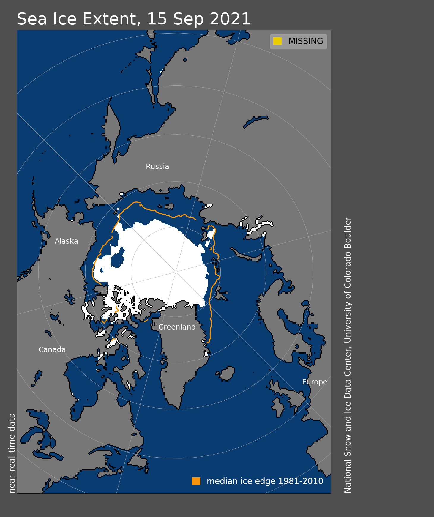
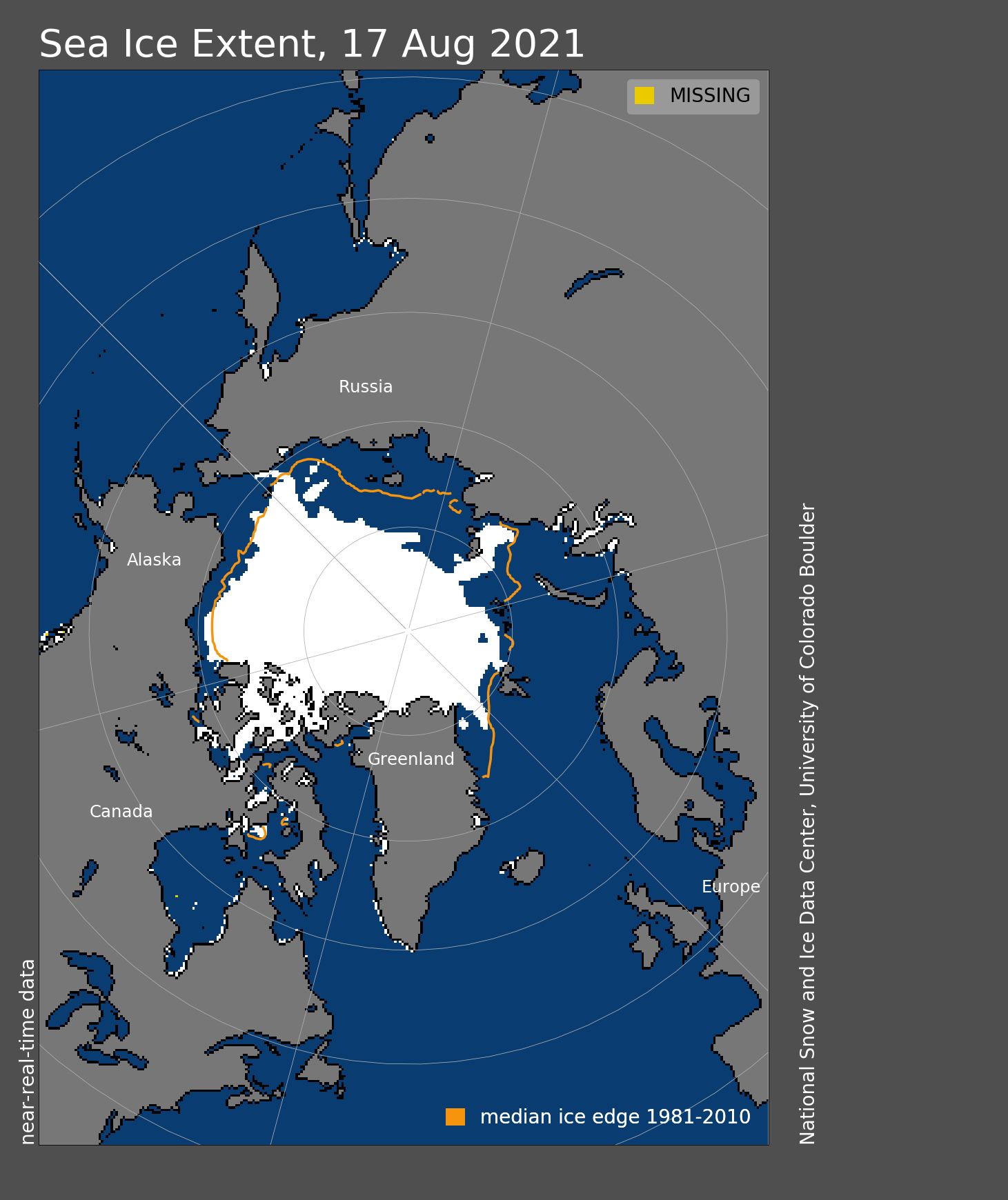
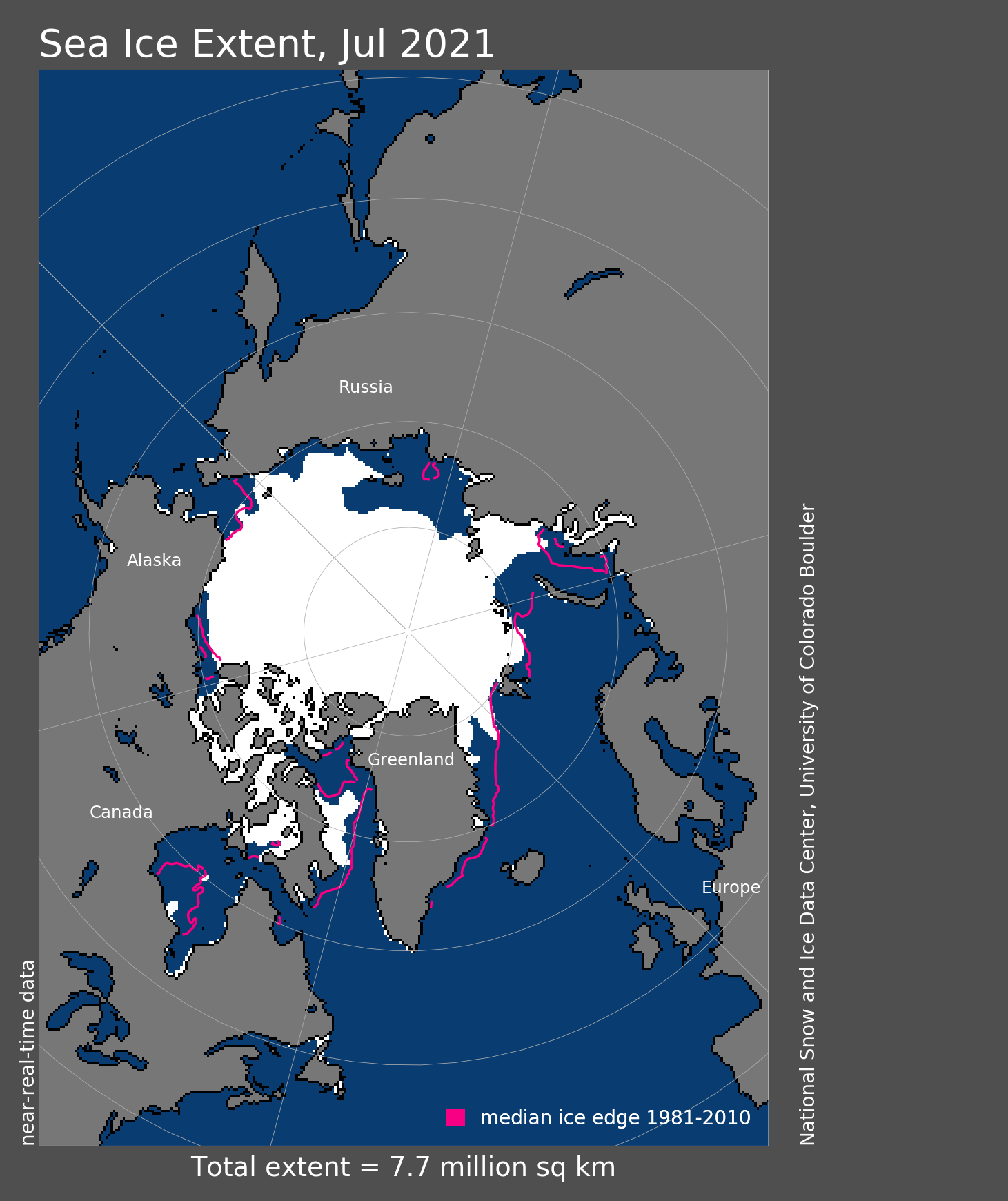
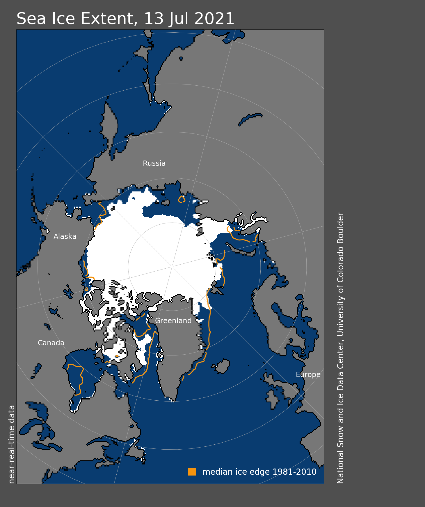
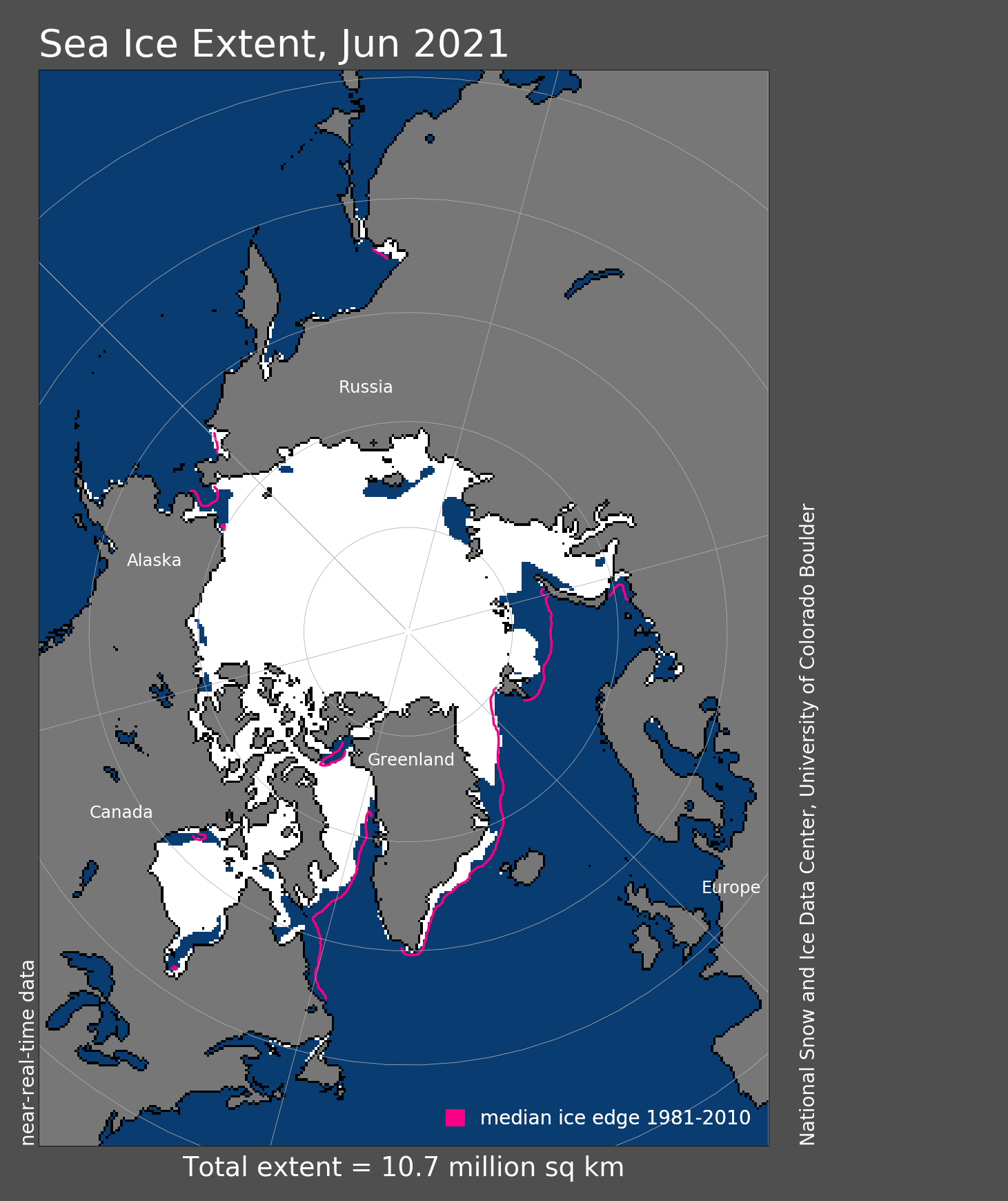
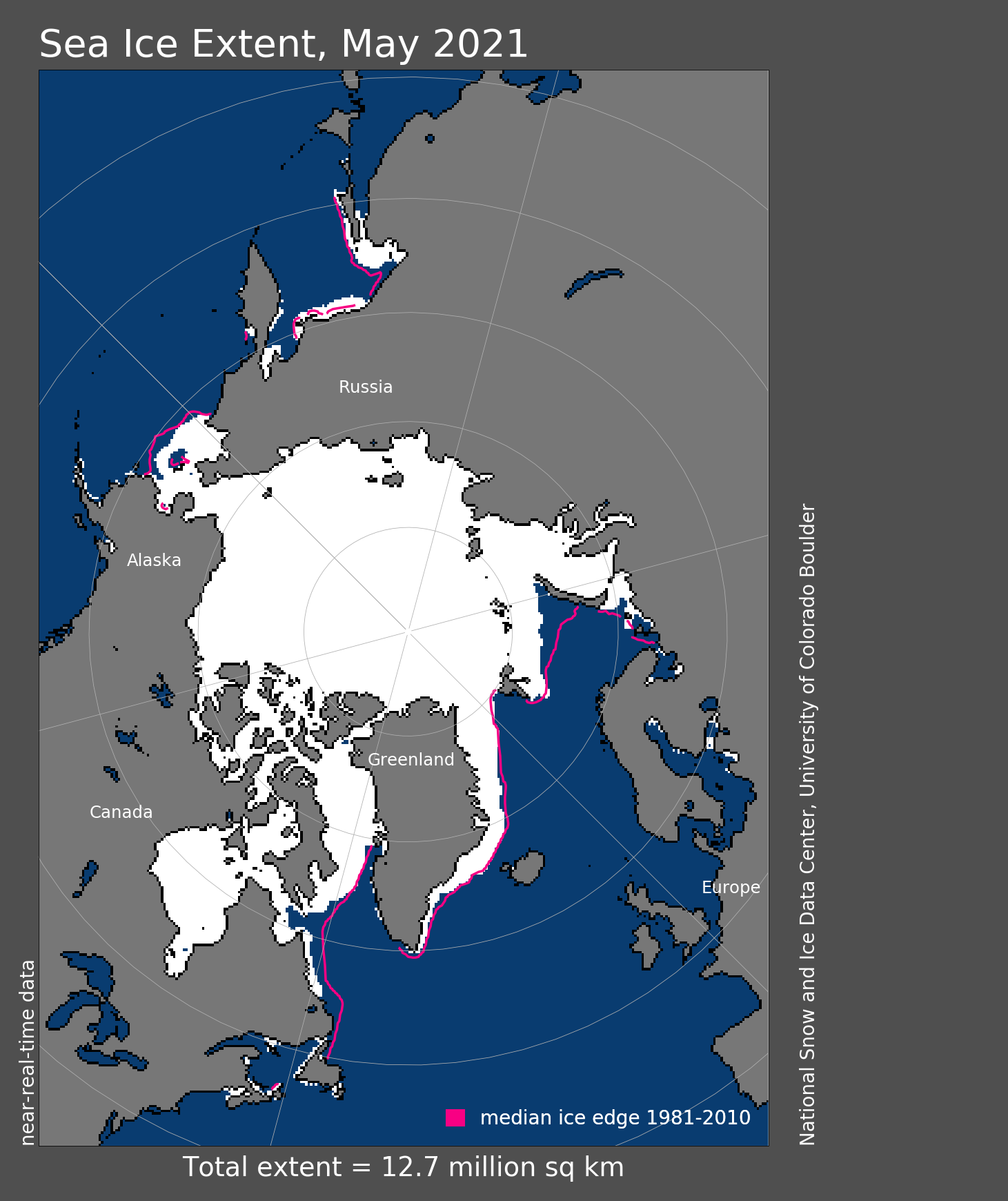
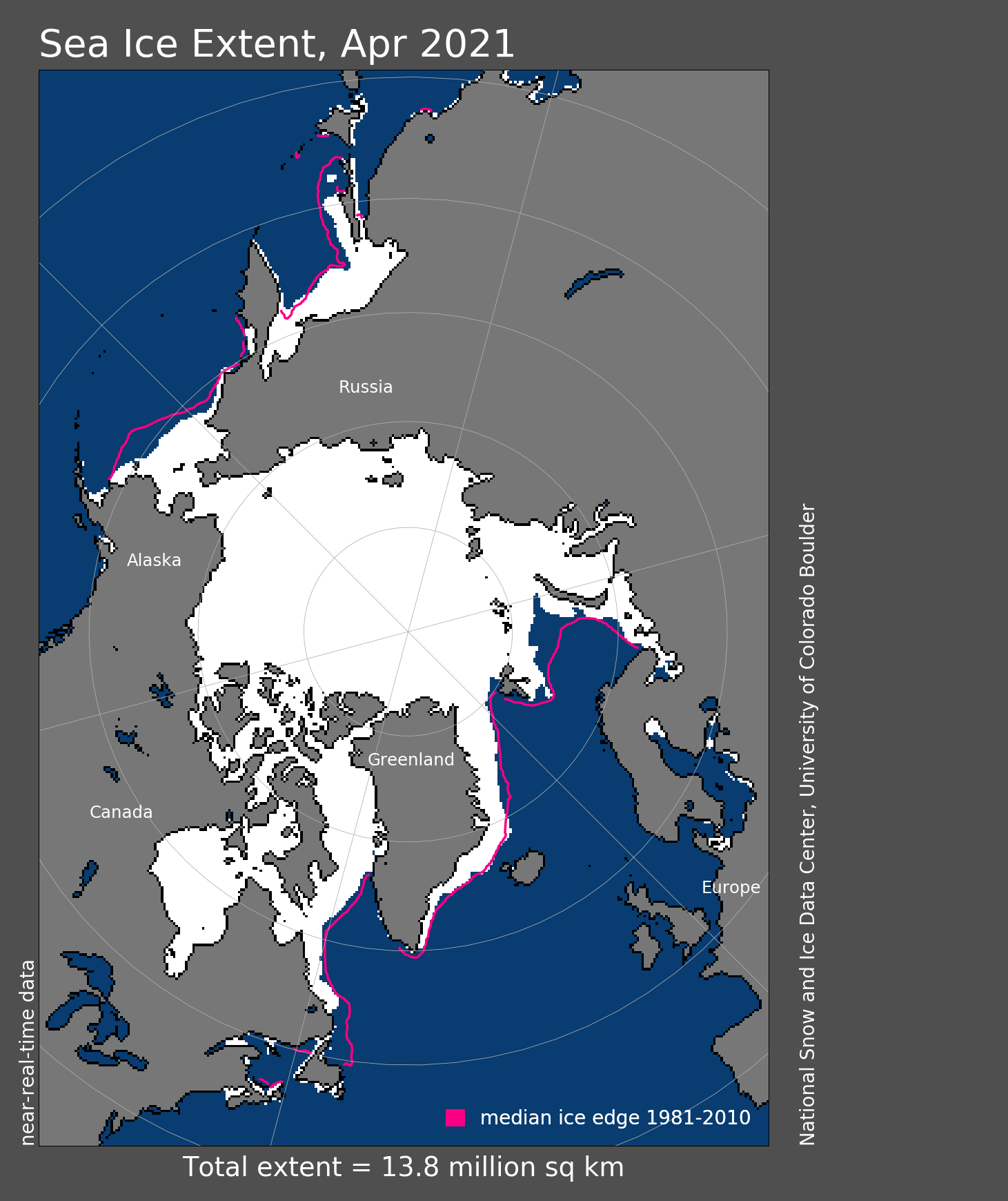
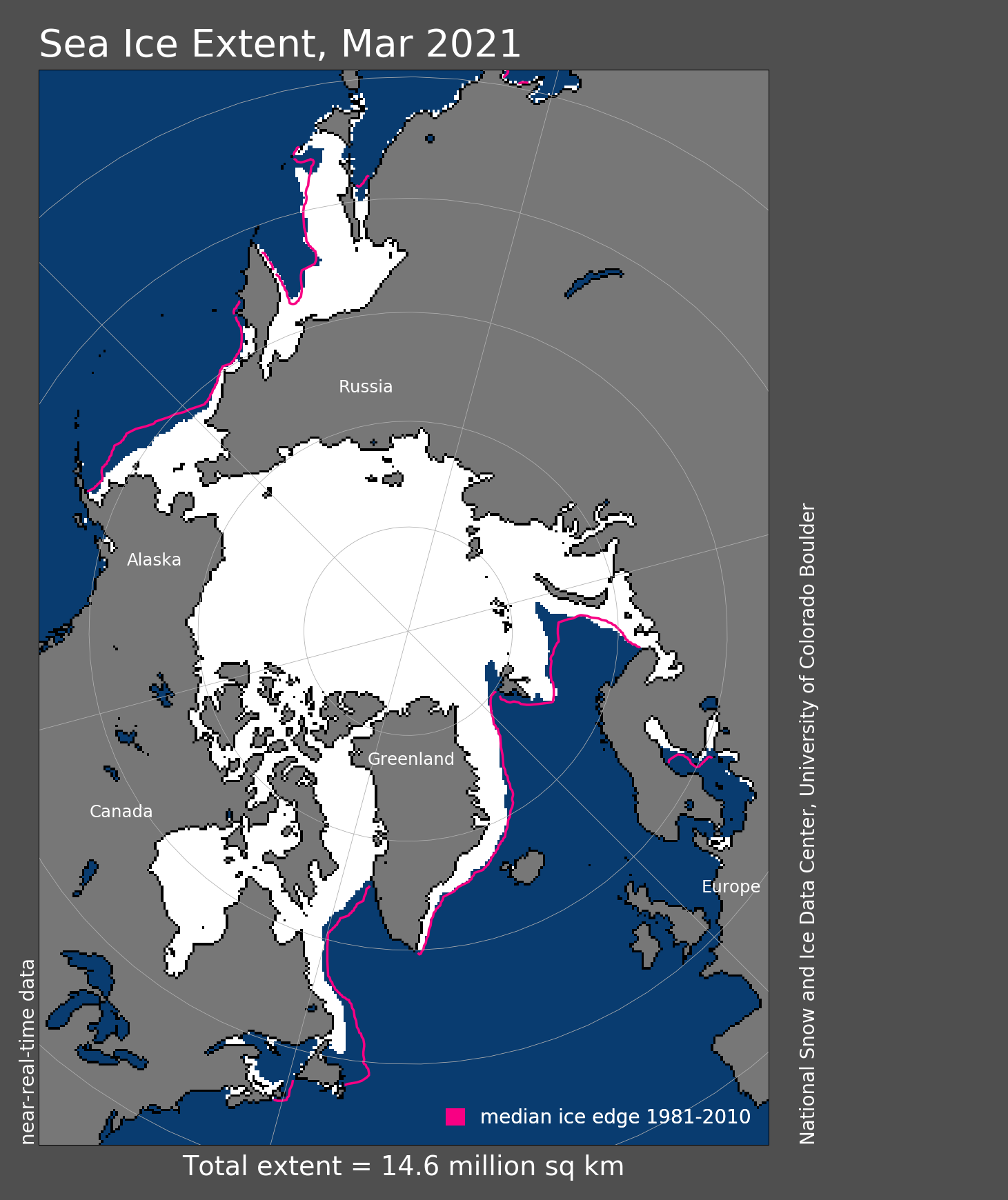
Figure 1. Arctic sea ice extent for May 2021 was 12.66 million square kilometers (4.89 million square miles). The magenta line shows the 1981 to 2010 average extent for that month. Sea Ice Index data. About the data

Credit: National Snow and Ice Data Center
High-resolution image

Arctic sea ice extent continued the slow pace of seasonal decline observed in April, leading to an average extent for May 2021 of 12.66 million square kilometers (4.89 million square miles). This was 740,000 square kilometers (286,000 square miles) above the record low for the month set in 2016 and 630,000 square kilometers (243,000 square miles) below the 1981 to 2010 average. The average extent for the month ranks ninth lowest in the passive microwave satellite record. The ice edge is near its average location most everywhere in the Arctic Ocean except in the Labrador Sea and east of Novaya Zemlya. Nevertheless, large polynyas have formed, notably north of the New Siberian Islands and east of Severnaya Zemlya. Open water areas have also developed near the coast in the southern Beaufort Sea and west of Utqiaġvik, Alaska (formerly Barrow). Overall, ice retreat during May occurred primarily in the Bering and Barents Seas, the Sea of Okhotsk and within the Laptev Sea.

Conditions in context

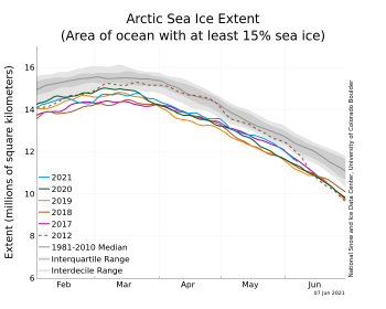
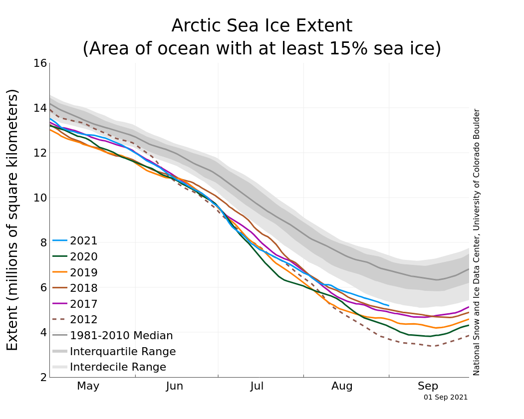
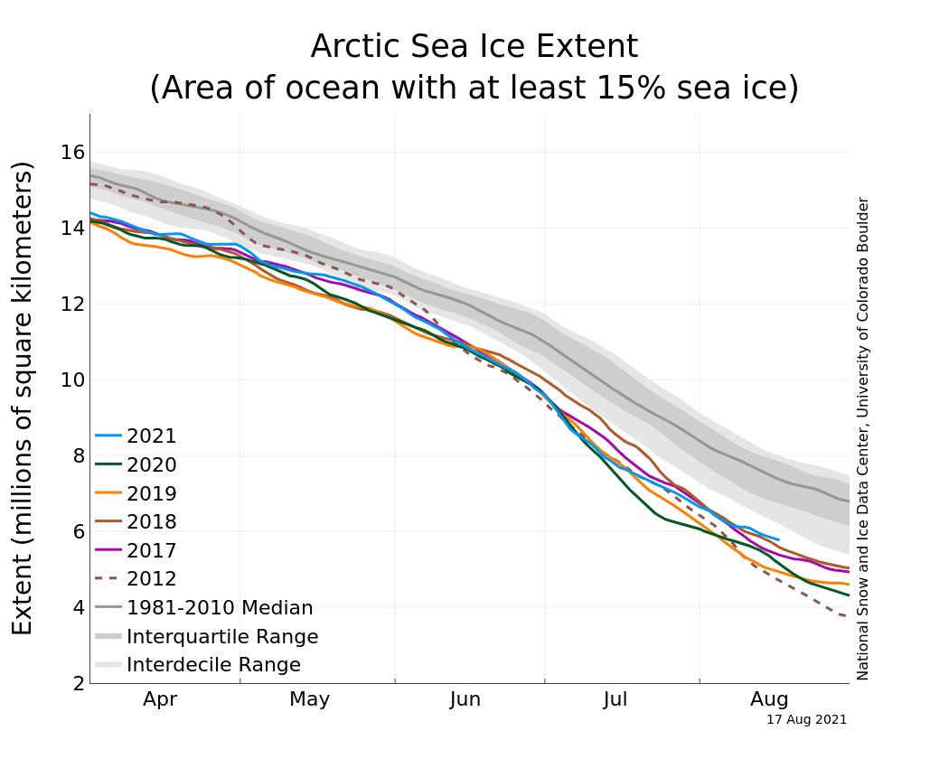
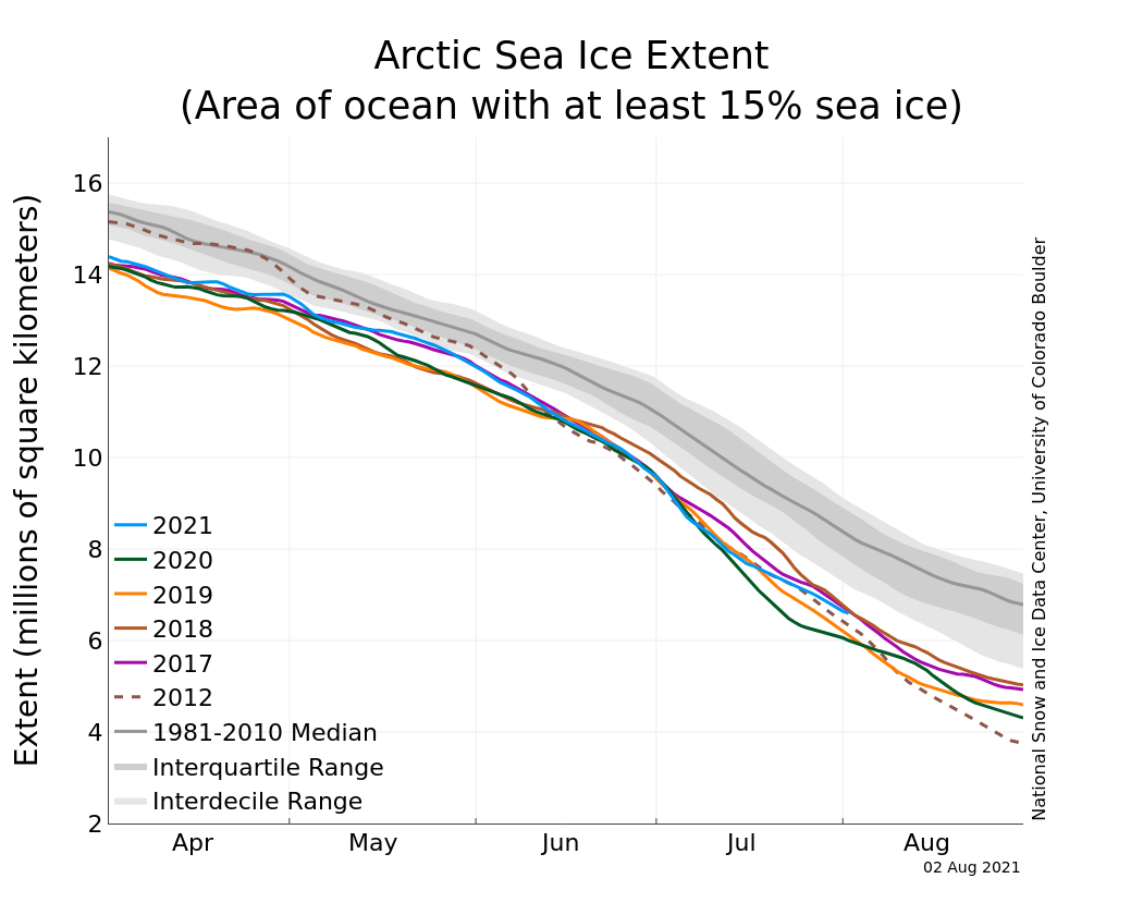
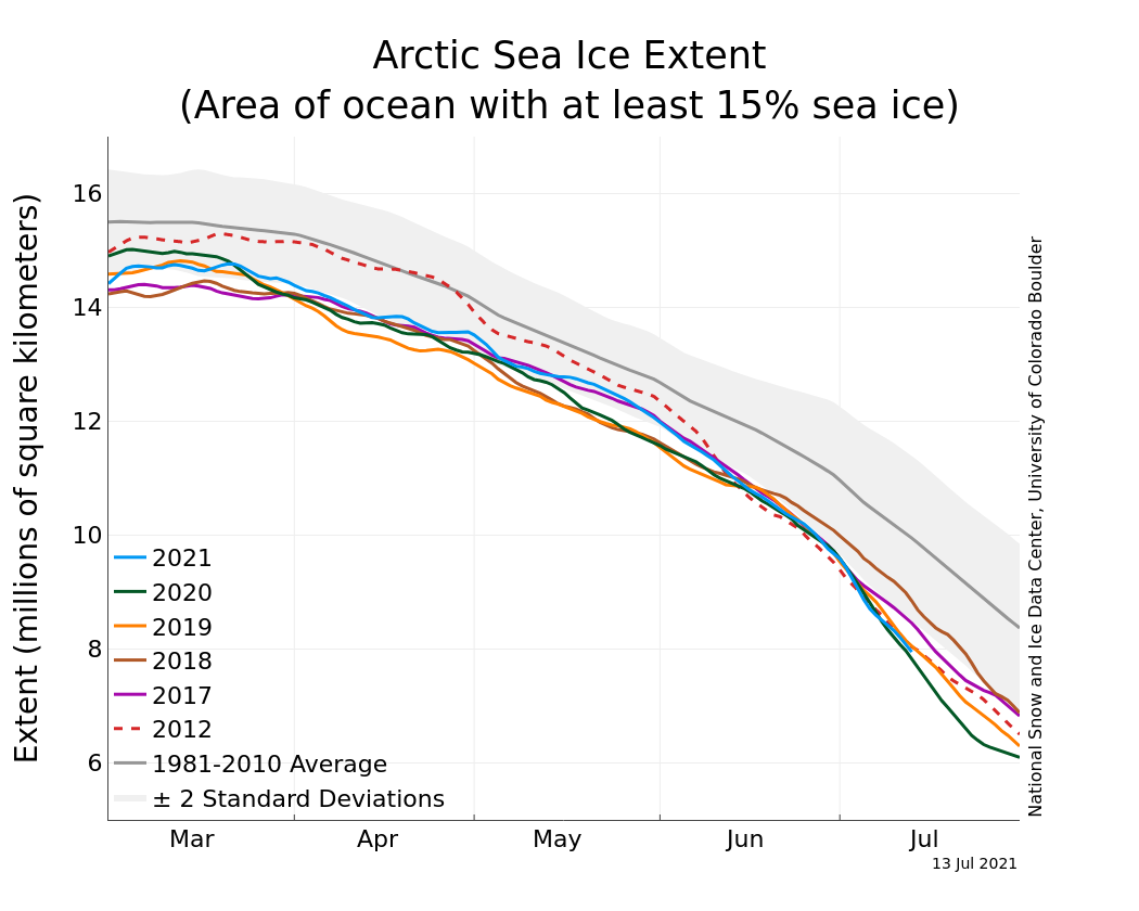
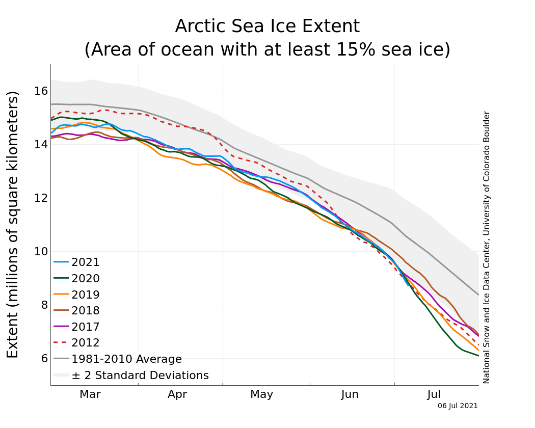
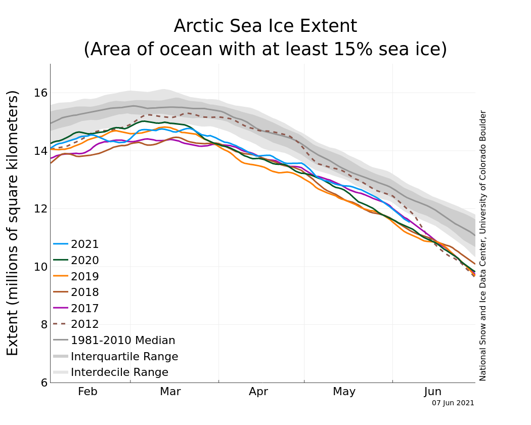
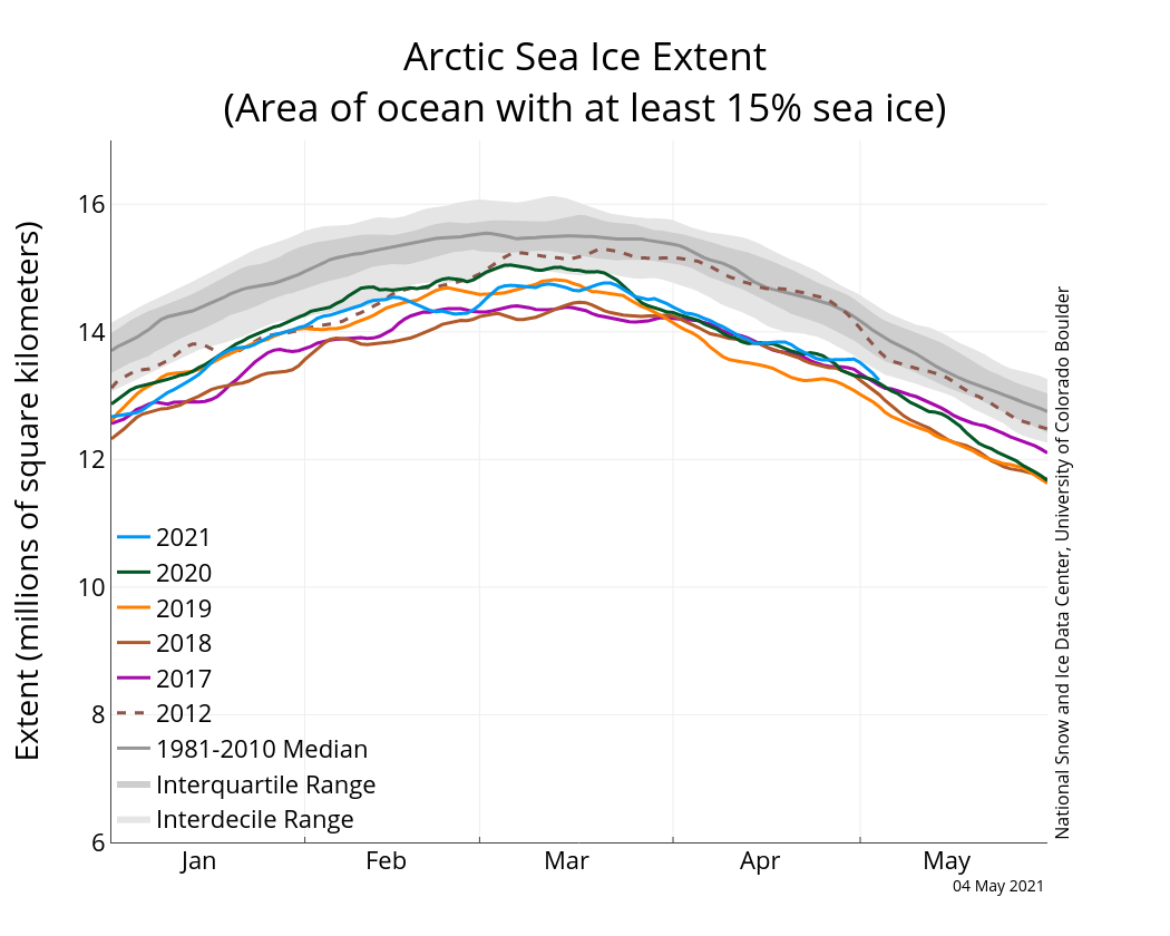
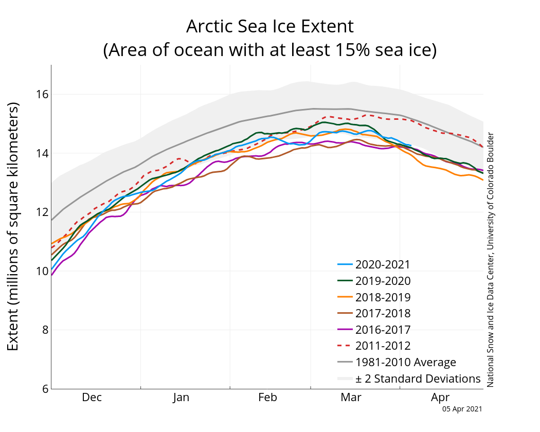
Figure 2a. The graph above shows Arctic sea ice extent as of June 7, 2021, along with daily ice extent data for four previous years and the record low year. 2021 is shown in blue, 2020 in green, 2019 in orange, 2018 in brown, 2017 in magenta, and 2012 in dashed brown. The 1981 to 2010 median is in dark gray. The gray areas around the median line show the interquartile and interdecile ranges of the data. Sea Ice Index data.

Credit: National Snow and Ice Data Center
High-resolution image

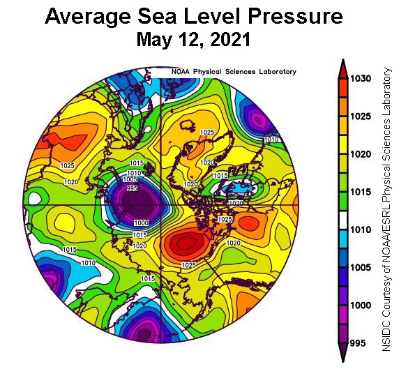
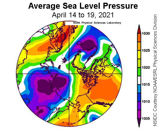
Figure 2b. This plot shows average sea level pressure in the Arctic in millibars on May 12, 2021. Yellows and reds indicate high air pressure; blues and purples indicate low pressure.

Credit: NSIDC courtesy NOAA Earth System Research Laboratory Physical Sciences Laboratory
High-resolution image

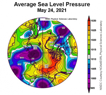
Figure 2c. This plot shows average sea level pressure in the Arctic in millibars on May 24, 2021. Yellows and reds indicate high air pressure; blues and purples indicate low pressure.

Credit: NSIDC courtesy NOAA Earth System Research Laboratory Physical Sciences Laboratory
High-resolution image

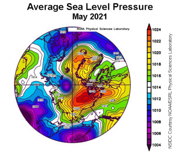
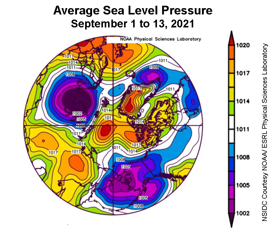
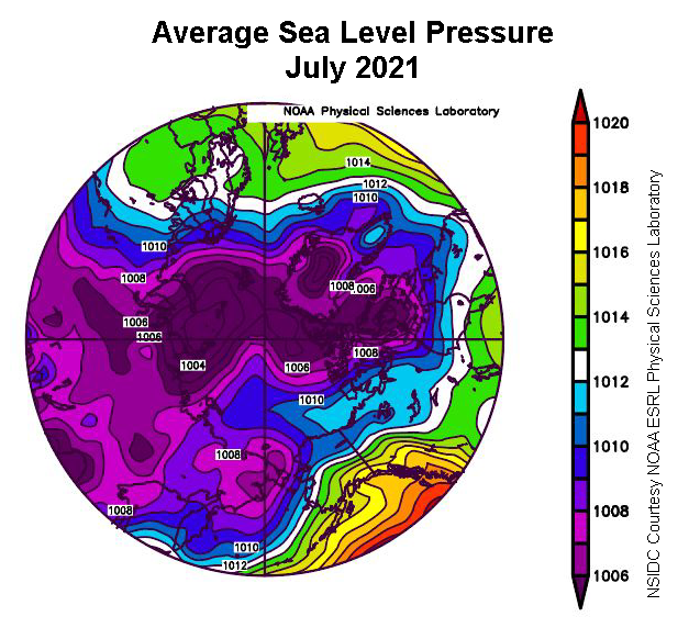
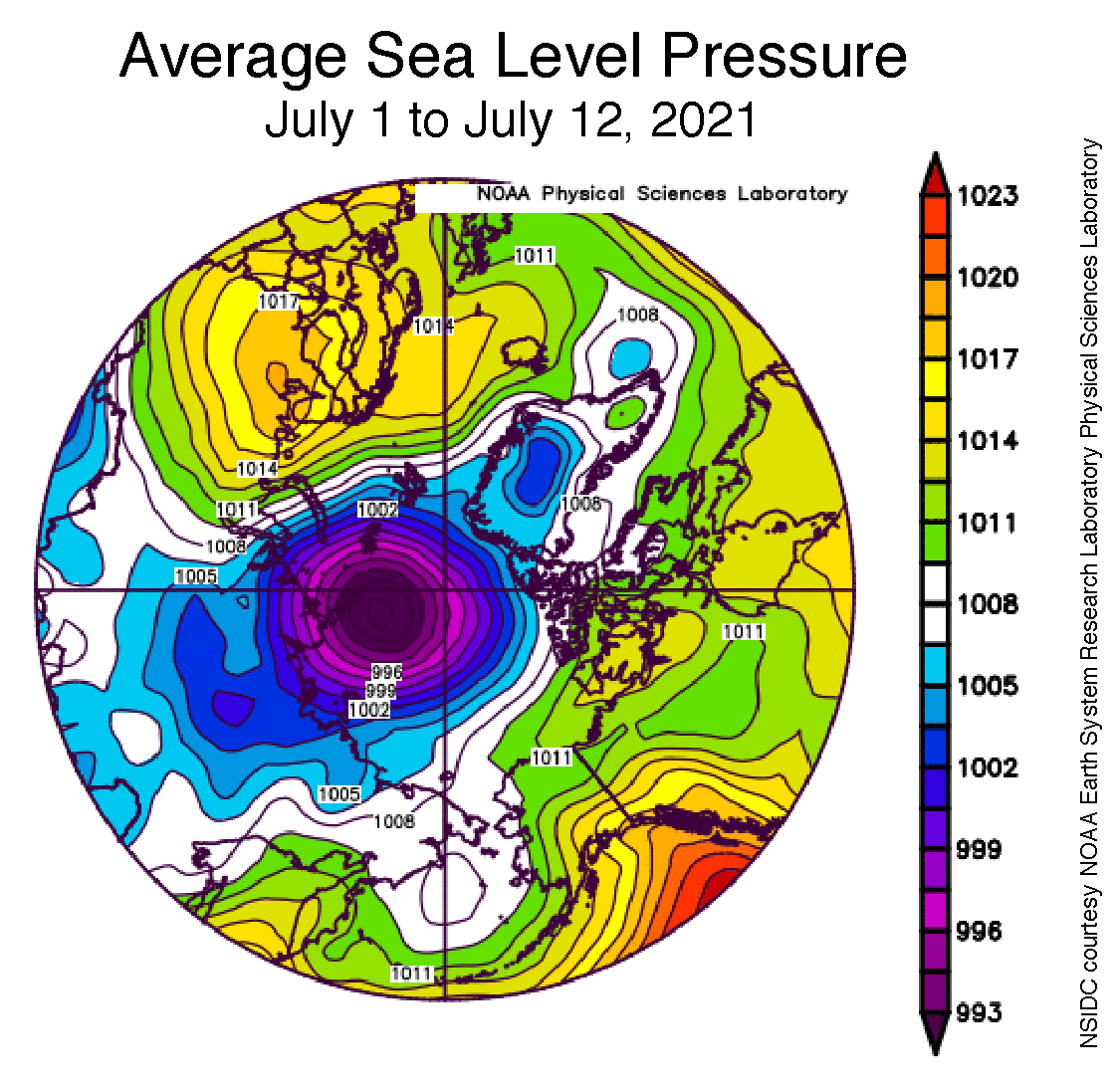
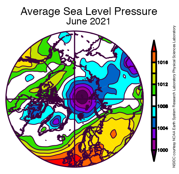
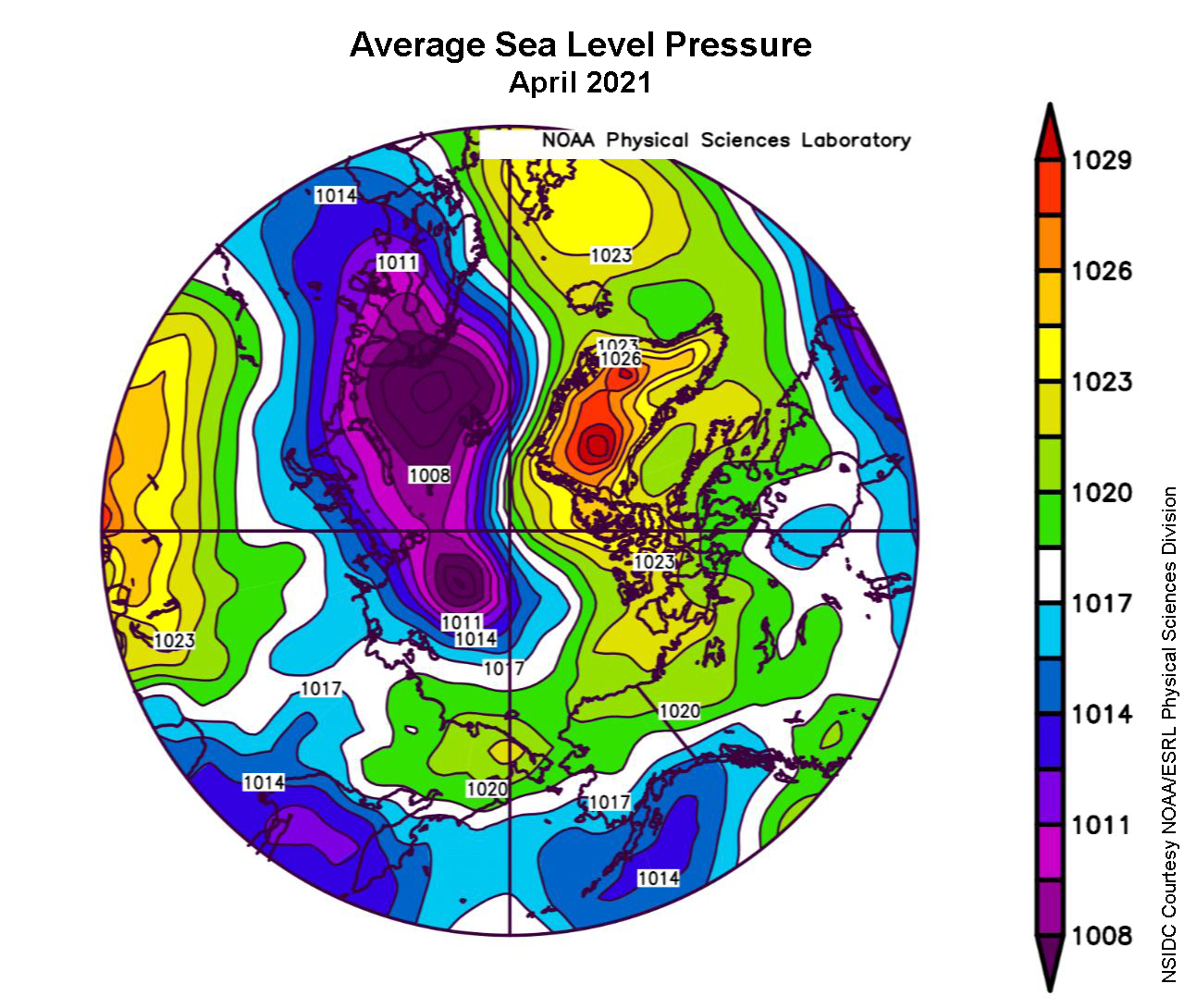
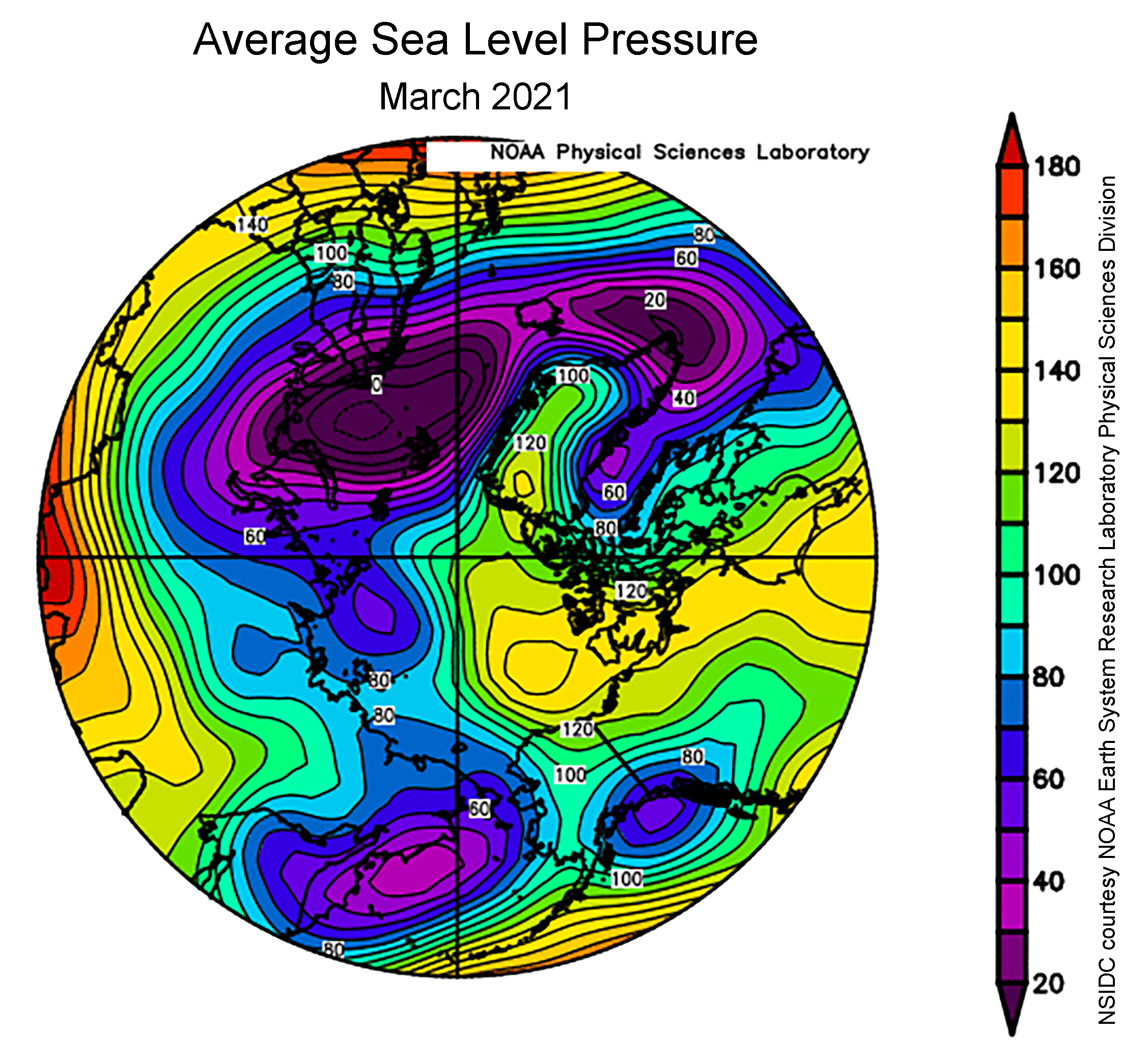
Figure 2d. This plot shows average sea level pressure in the Arctic in millibars for May 2021. Yellows and reds indicate high air pressure; blues and purples indicate low pressure.

Credit: NSIDC courtesy NOAA Earth System Research Laboratory Physical Sciences Laboratory
High-resolution image

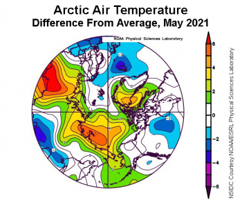
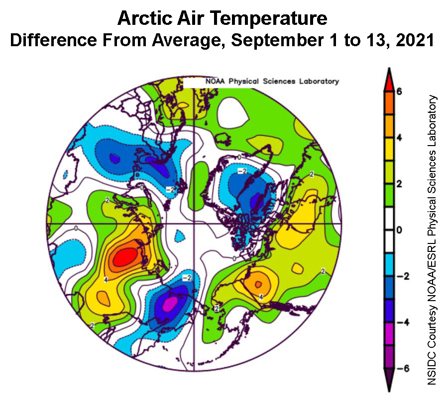
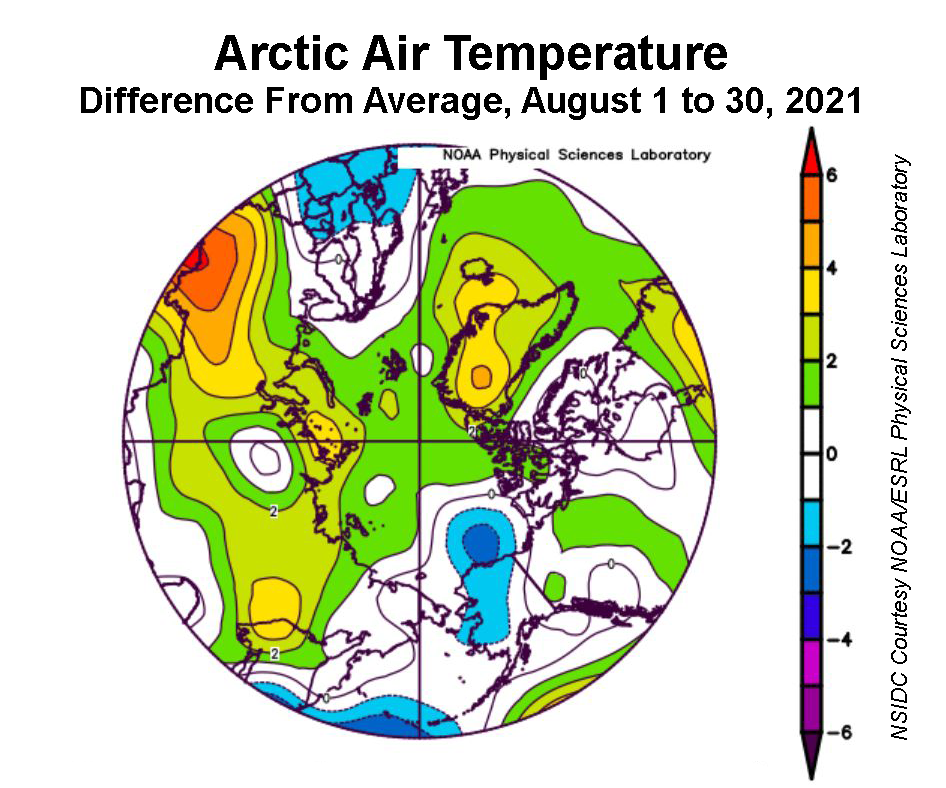
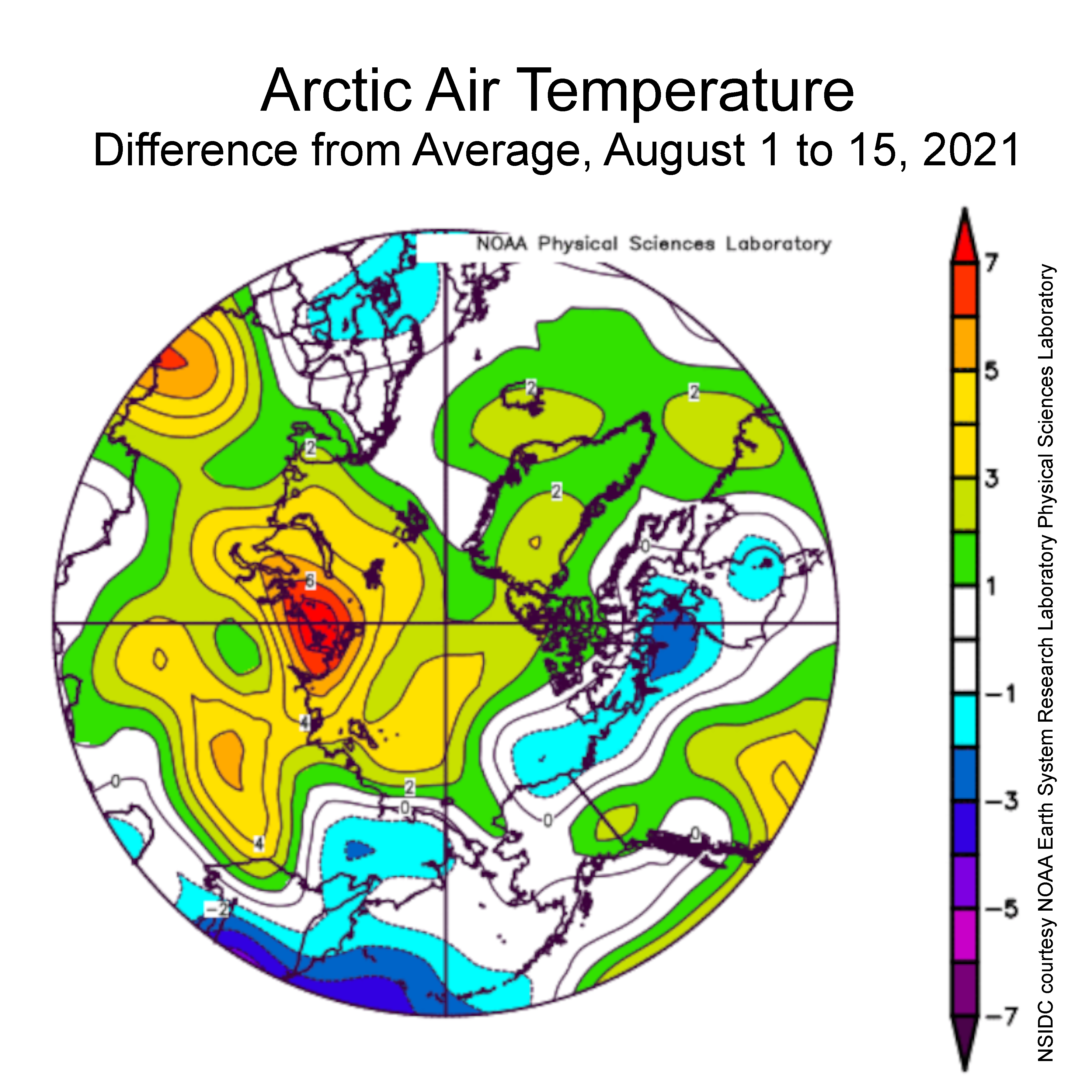
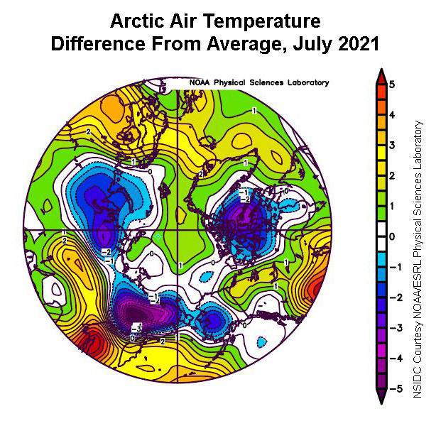
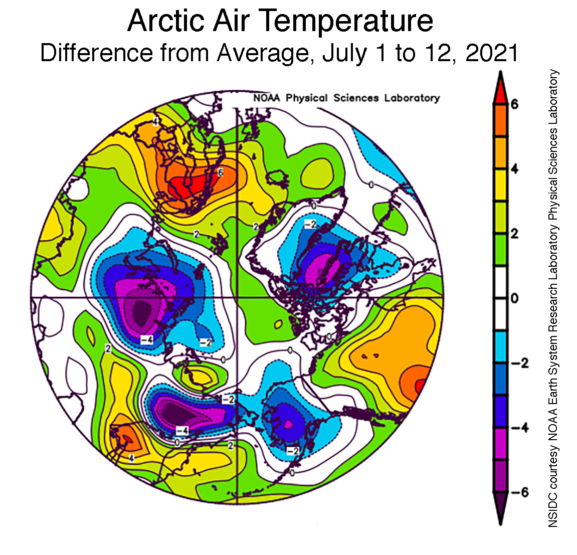
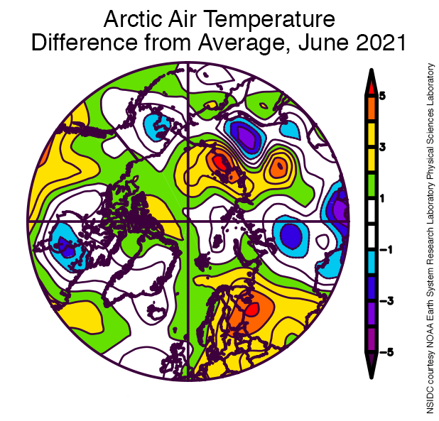
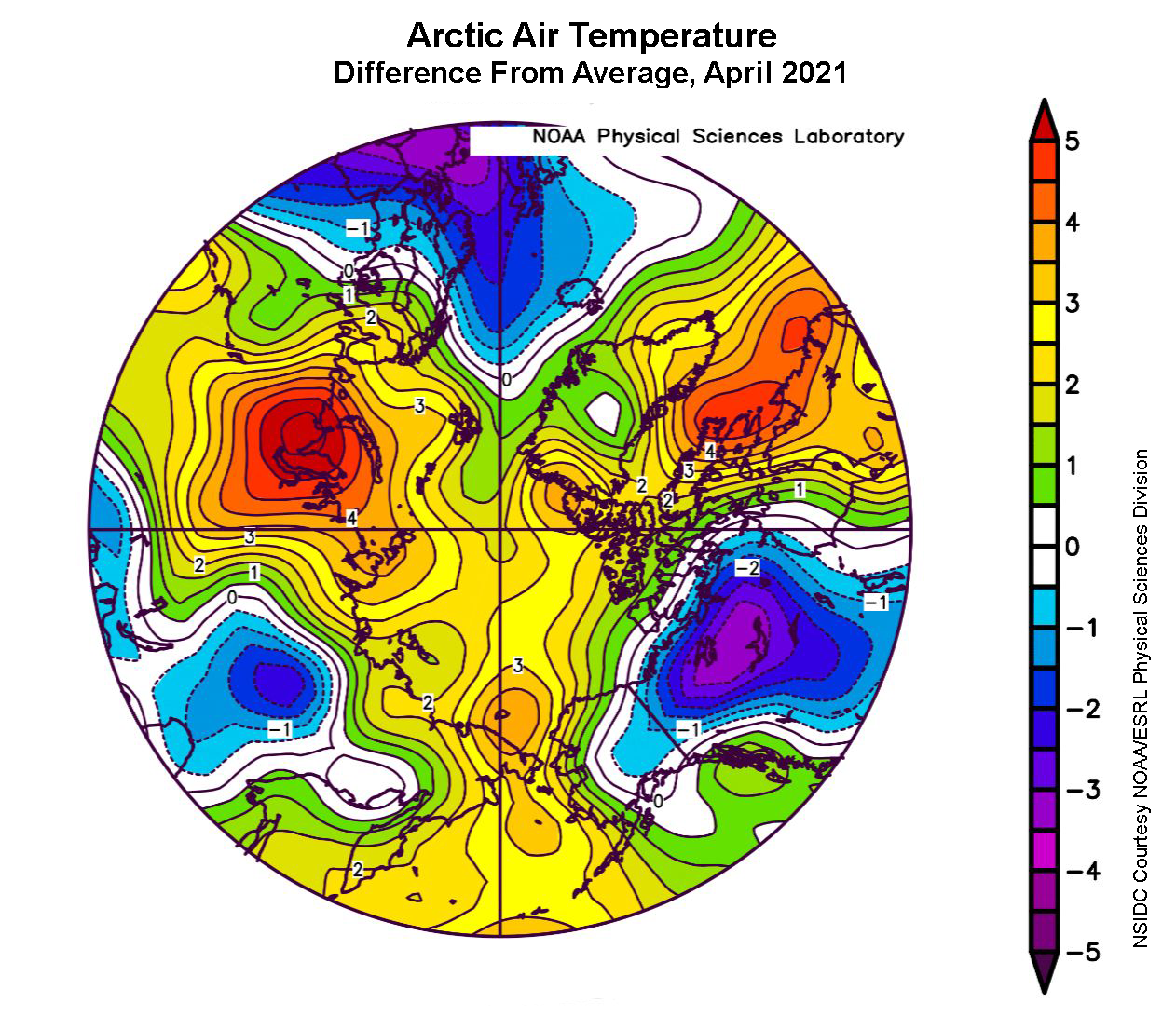
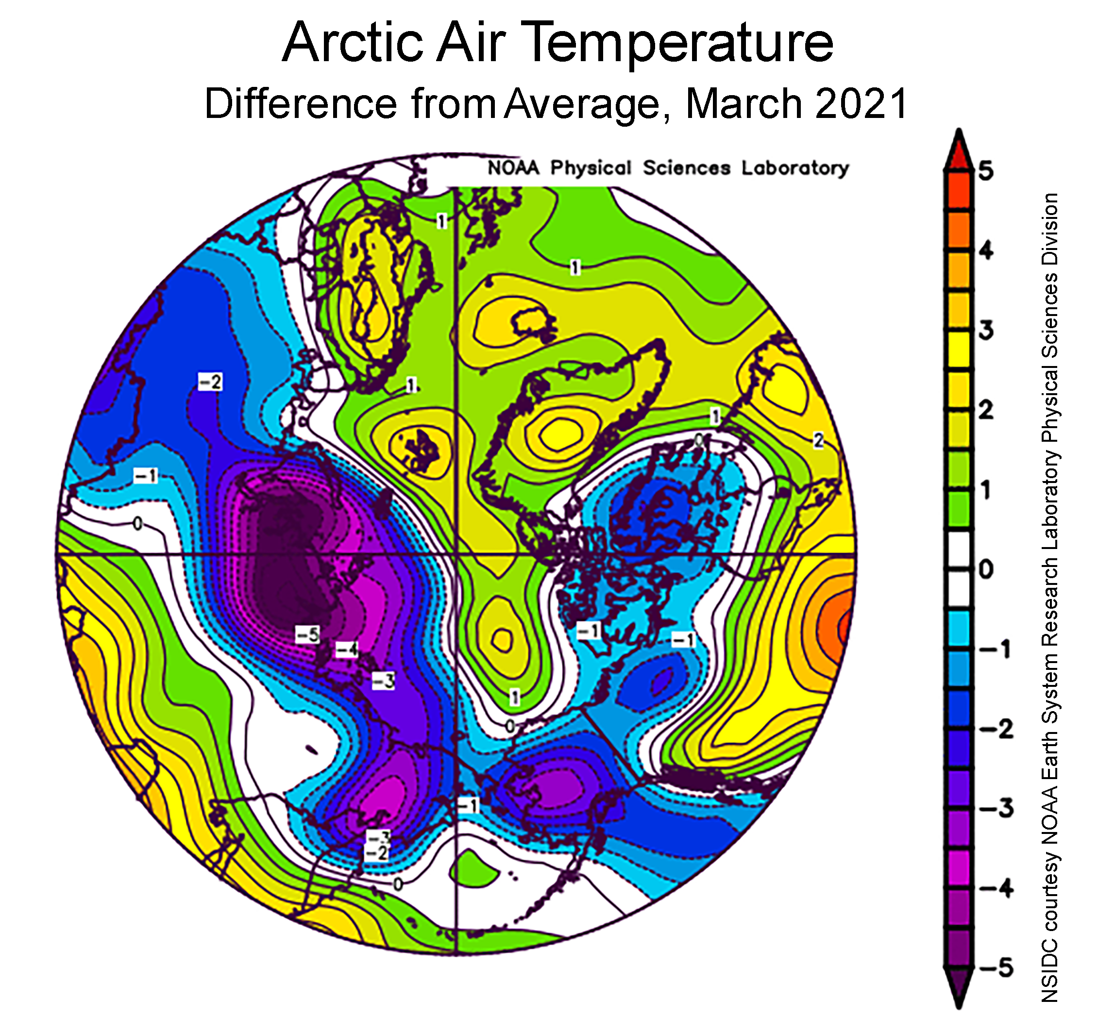
Figure 2e. This plot shows the departure from average air temperature in the Arctic at the 925 hPa level, in degrees Celsius, for May 2021. Yellows and reds indicate higher than average temperatures; blues and purples indicate lower than average temperatures.

Credit: NSIDC courtesy NOAA Earth System Research Laboratory Physical Sciences Laboratory
High-resolution image

The slow pace of sea ice loss this month (Figure 2a) can be explained in large part by a series of storms that migrated over the pole during May. The first storm split from a system over the Barents Sea and then slowly intensified over the central Arctic Ocean before reaching peak intensity (1007 hPa) north of Severnaya Zemlya on May 4. This was followed by another storm tracking northward from Europe, reaching peak intensity (sea level pressure of 987 hPa) over Severnaya Zemlya on May 12 and then joining with another storm that formed over Siberia on May 16 (Figure 2b). The strongest of the storms in terms of minimum central pressure (984 hPa) pressure, achieved on May 24, once again was located over Severnaya Zemlya and resulted from the merging of two systems moving in from the Barents Sea (Figure 2c).

As a result of the May storms, sea level pressure was lower than average by 6hPa centered just south of the pole at about 90 degrees E longitude. This was coupled with sea level pressure of 6 to 8 hPa above average over Greenland and the Canadian Arctic Archipelago extending into the northern Beaufort and Chukchi Seas (Figure 2d). Combined, this sea level pressure pattern fostered cold air spilling out of the Arctic Ocean into the North Atlantic and warm air flowing from the south over eastern Russia, leading to monthly averaged air temperatures at the 925 hPa level 1 to 4 degrees Celsius (2 to 7 degrees Fahrenheit) above average for this time of year over much of the Arctic Ocean, but up to 6 degrees Celsius (11 degrees Fahrenheit) above average along the coast of the Laptev and East Siberian Seas (Figure 2e). By contrast, temperatures were below average east of Greenland and around Svalbard. Wind patterns also explain the opening of the ice cover around Franz Joseph Land, the New Siberian Islands, and in the southern Beaufort Sea.

May 2021 compared to previous years

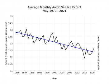
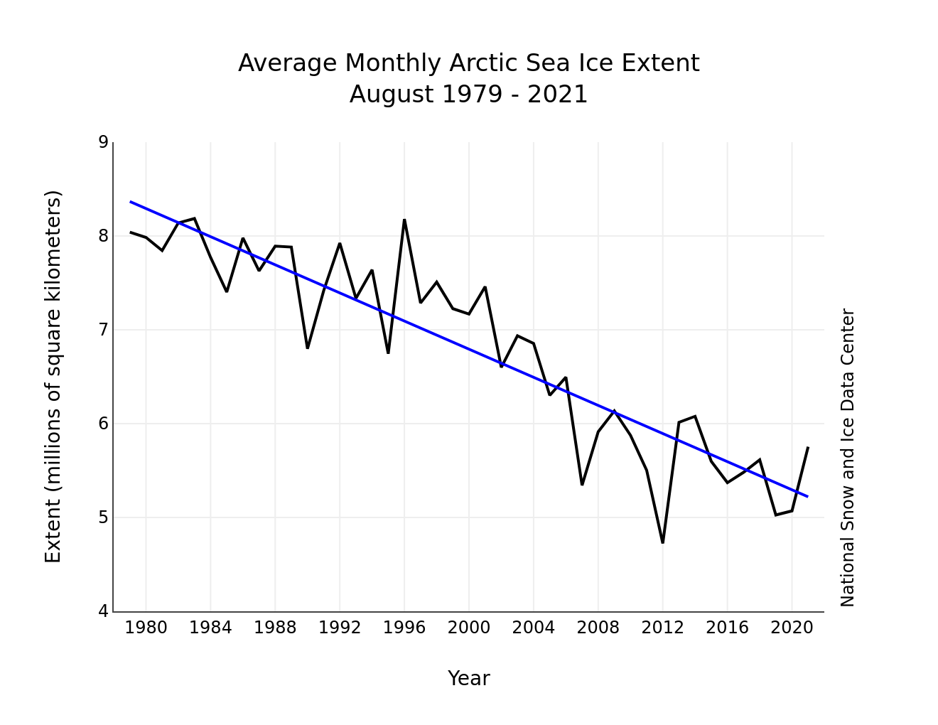
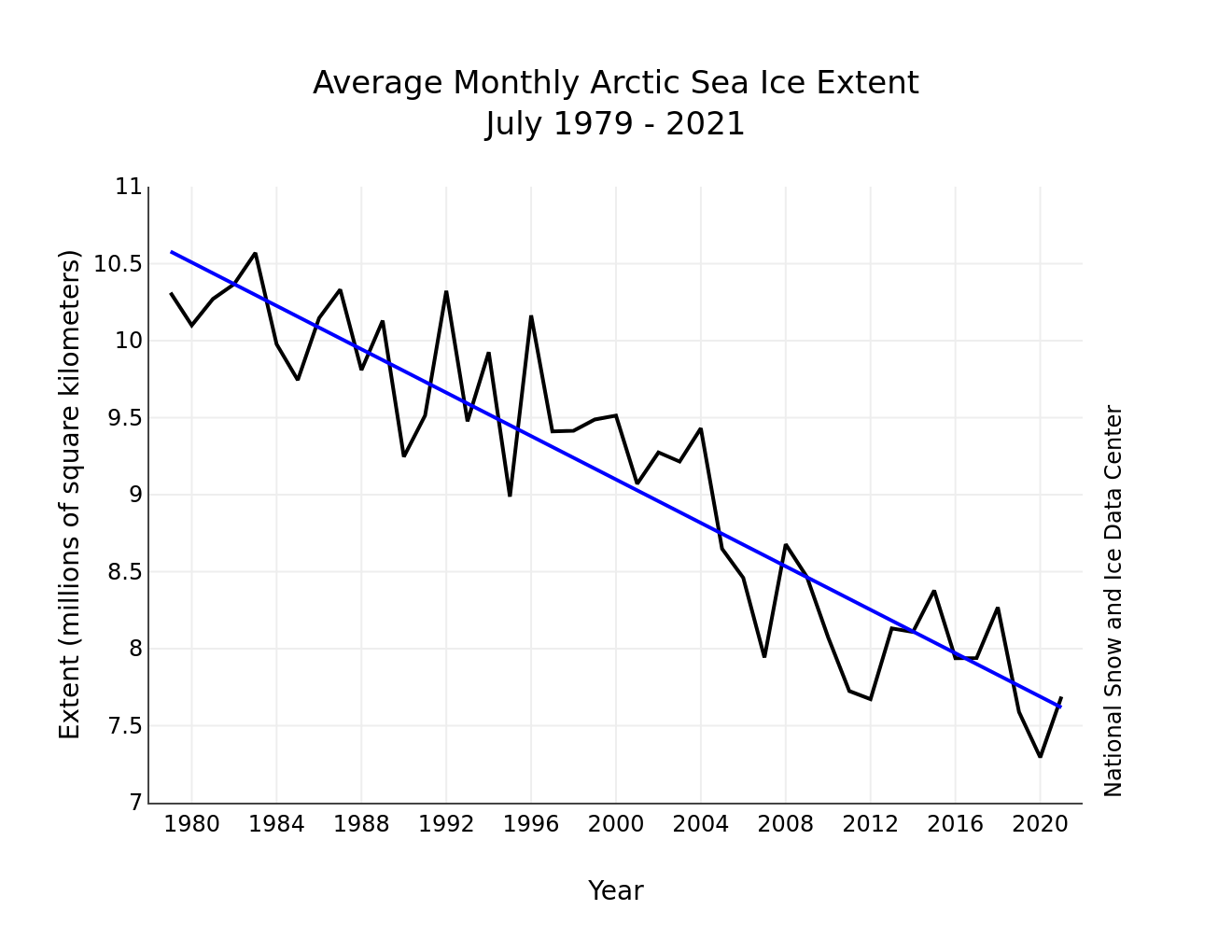
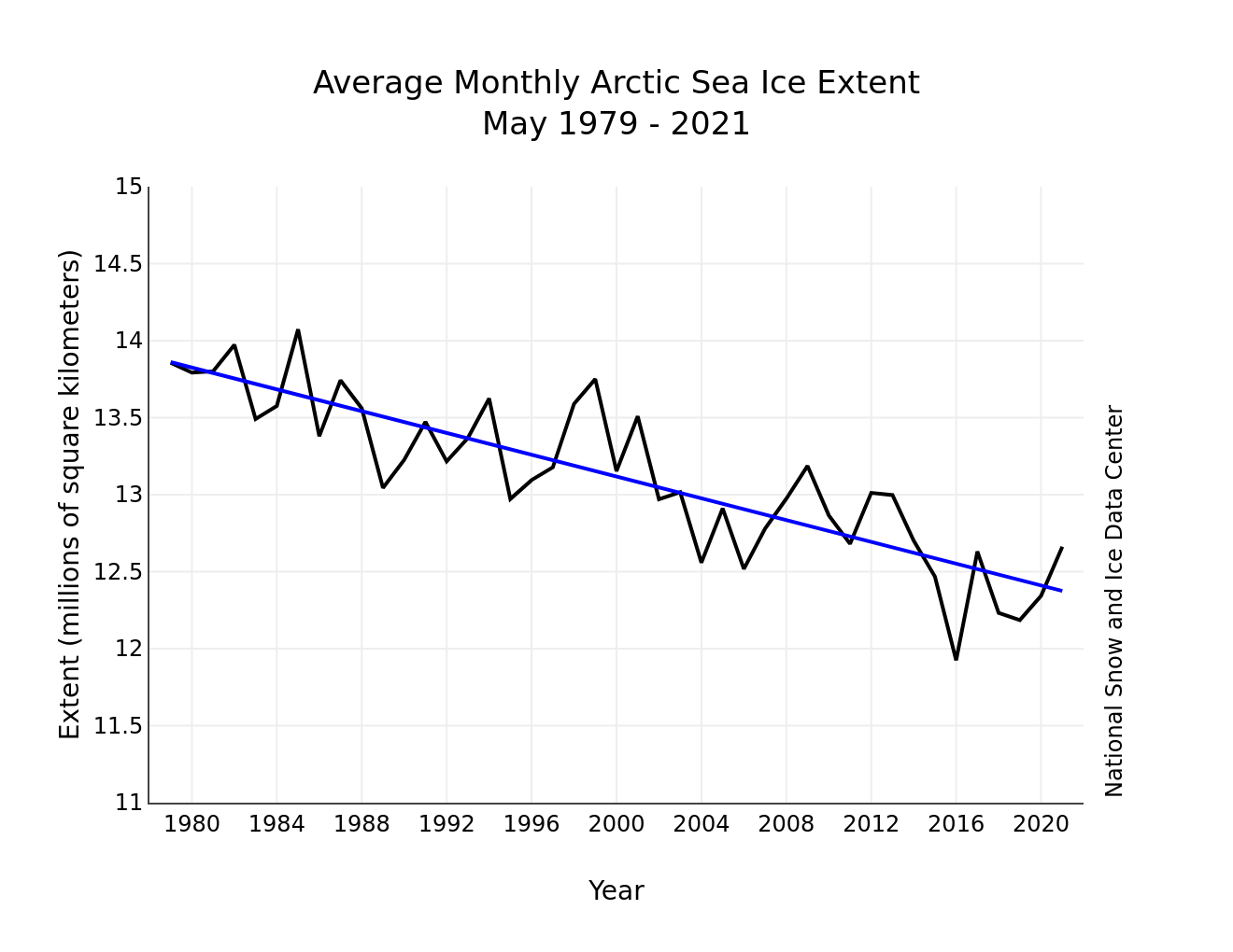
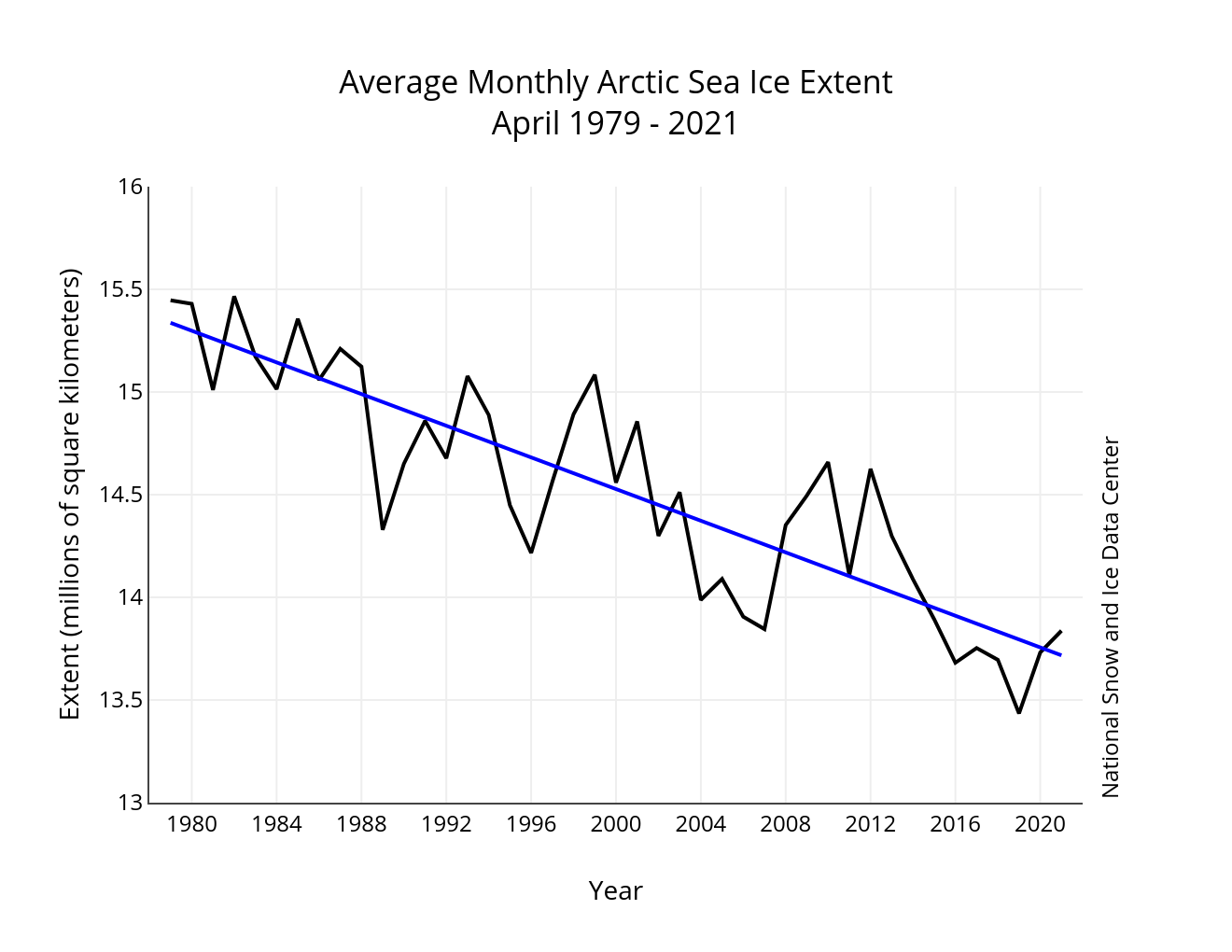
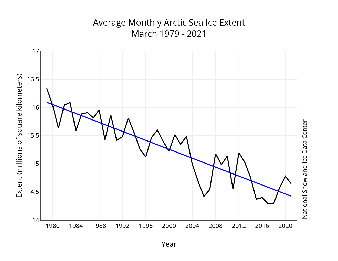
Figure 3. Monthly May ice extent for 1979 to 2021 shows a decline of 2.7 percent per decade.

Credit: National Snow and Ice Data Center
High-resolution image

Overall, the pace of ice loss was slower than average, leading to only the ninth lowest May extent during the satellite data record. Through 2021, the linear rate of decline for May sea ice extent, relative to the 1981 to 2020 average extent, is 2.7 percent per decade. This corresponds to 35,400 square kilometers (13,700 square miles) per year, about the size of the state of Maine. The cumulative May ice loss over the 43-year satellite record is 1.49 million square kilometers (575,000 square miles), based on the difference in linear trend values in 2021 and 1979. This is roughly twice the size of the state of Texas.

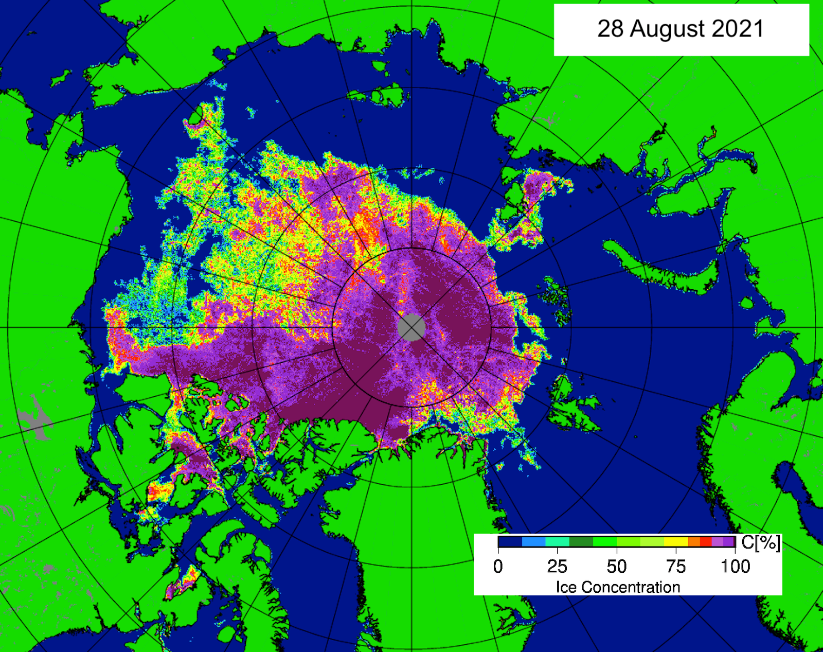
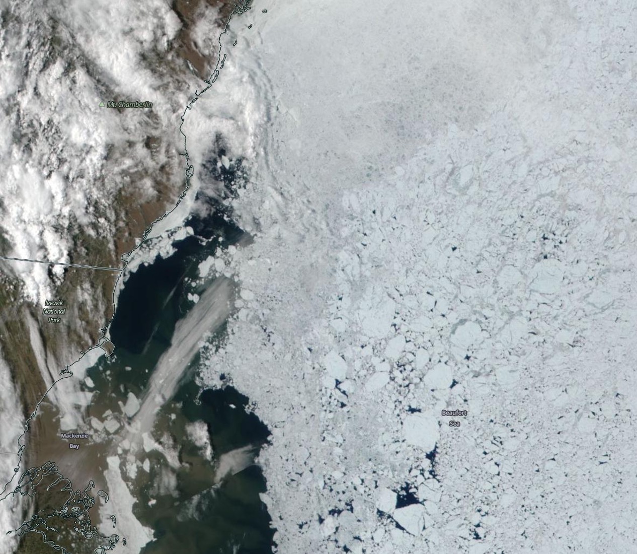
Capturing the break up in the Beaufort Sea

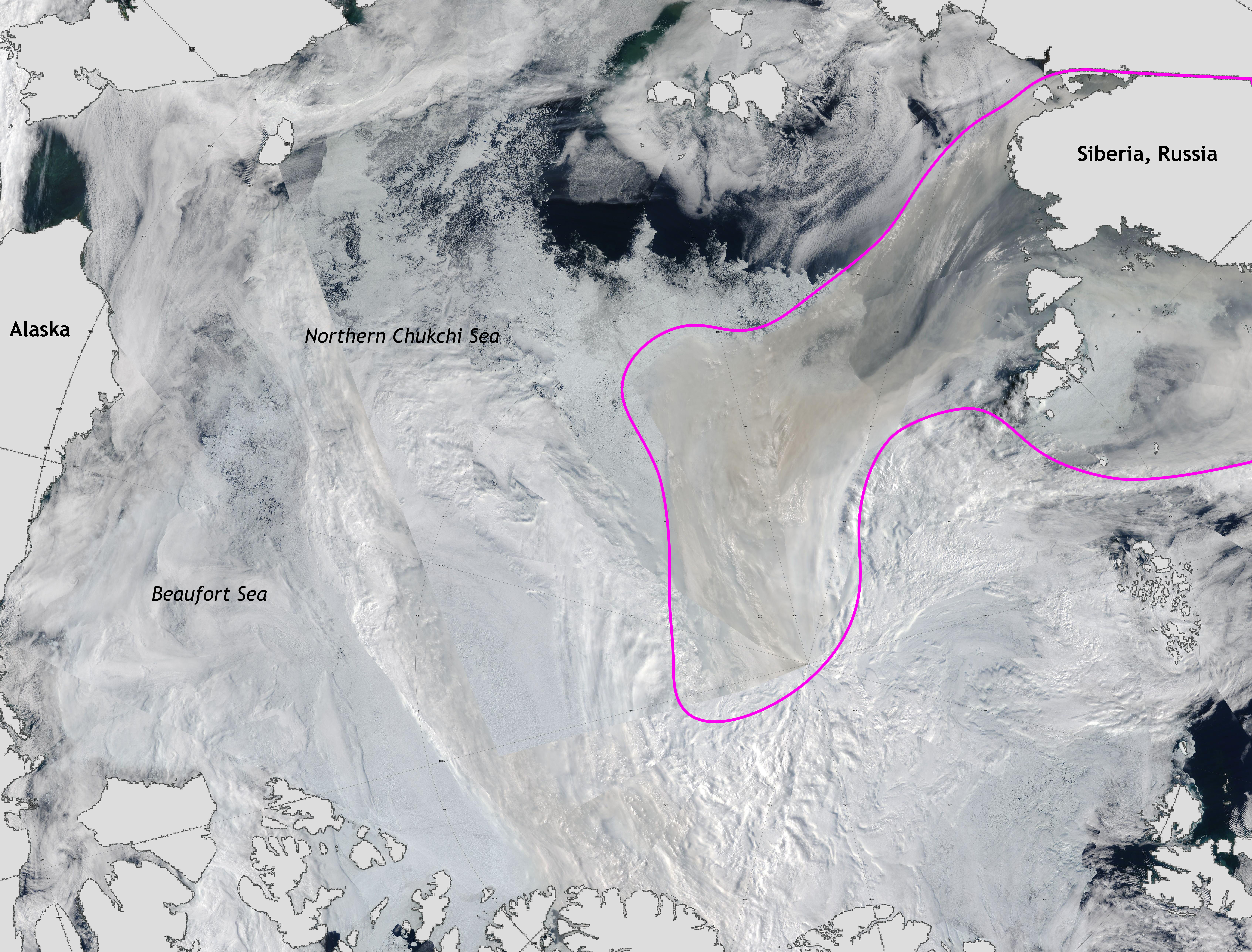
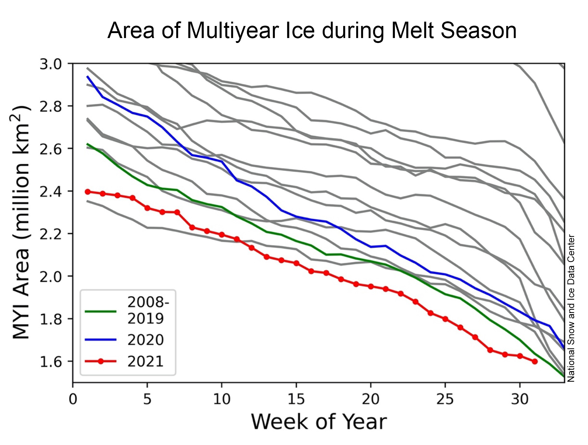
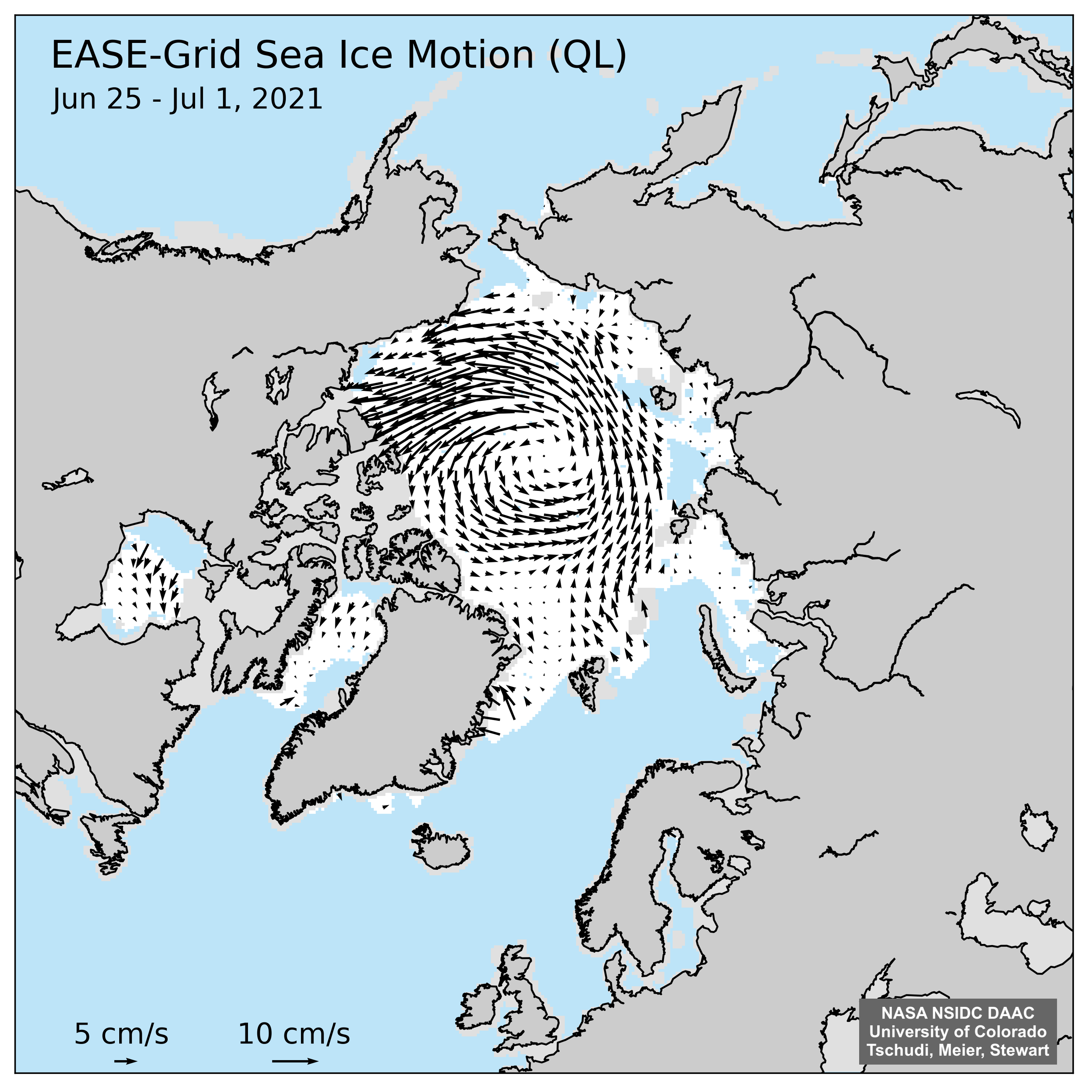
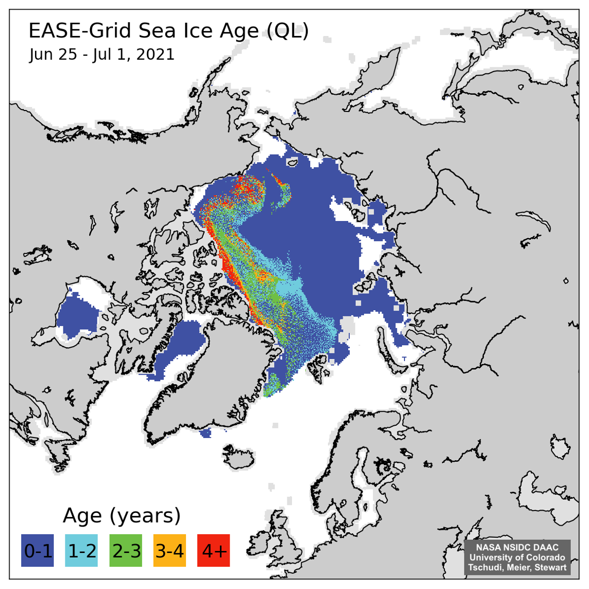
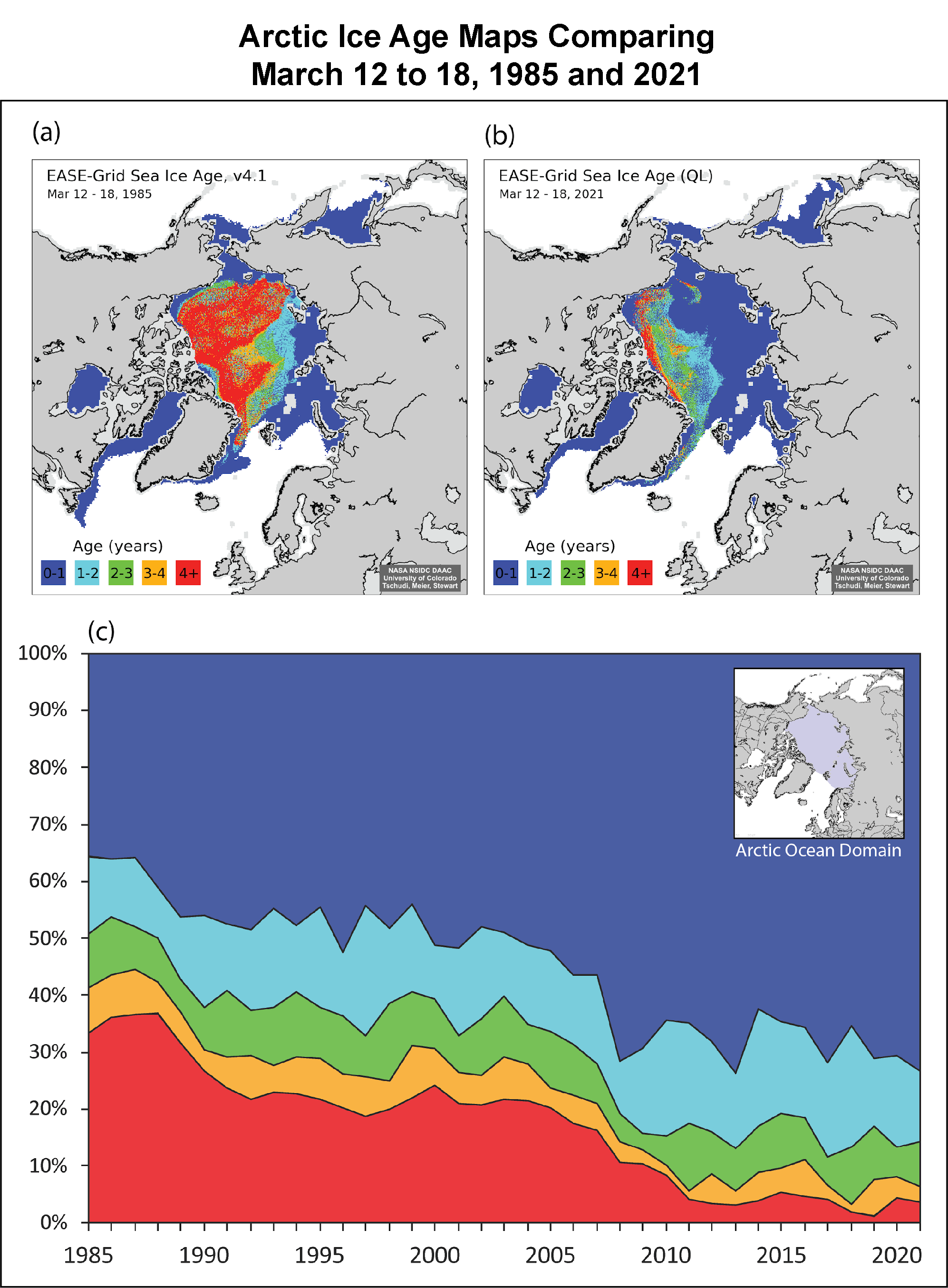
Visible wavelength imagery from the NASA Moderate Resolution Imaging Spectroradiometer (MODIS) provides the opportunity to track the ice breaking up in the southern Beaufort Sea this May; cloud cover was limited, offering decent views of the surface. Between April 25 and May 17, the pack ice started to move away from the landfast ice still attached to the coast, leading to open water and subsequent break up of the ice floes and partial break up of the landfast ice by mid-May. During the past winter, unusually high sea level pressure over the central Arctic Ocean resulted in unusually strong anticyclonic (clockwise) ice motion that drove a lot of fairly old ice from the central Arctic Ocean into the Beaufort Sea. Early break up of ice can enhance lateral and basal melt (at the underside of the ice) of the ice floes. This process can weaken the multiyear ice in the region and help to further deplete the Arctic of its multiyear ice. Large losses of multiyear ice in the region followed the unusually strong negative Arctic Oscillation winter of 2009 to 2010, which also featured a strong clockwise flow of the ice cover. More recently, analysis of Canadian ice charts by David Babb at the University of Manitoba suggests that between 2016 and 2020 on average 210,000 square kilometers (81,000 square miles) of multiyear ice now melts out each summer in the Beaufort Sea.

Are wavy jet stream winds wavier? Or not?

A new study takes a close look at an idea discussed several times in the Arctic Sea Ice News and Analysis (ASINA) reports—that Arctic Amplification, the observed strong warming in the Arctic region, driven in part by loss of Arctic sea ice, is affecting the shape and persistence of the jet stream. The polar front jet stream marks the boundary in the atmosphere between cold Arctic air and warmer mid-latitude air. Numerous studies have proposed that Arctic Amplification weakens the latitudinal temperature and atmospheric pressure gradient, manifested as a weaker and more sinuous jet stream. Since storms (low pressure systems) tend to form along the jet stream, weather in middle latitudes ought to become more variable, with large swings and more persistent patterns.

While the issue has long been controversial, the new study by James Screen, which was presented at the European Geophysical Union annual meeting in April, but has not yet been published, finds little evidence for this effect in climate model simulations and observations. In examining the past decade of observations, relationships that initially gave support to the idea have weakened. Even with far more open water conditions expected by 2050, the modeled effects of Arctic warming on the weather patterns at lower latitudes appear to be minor. The response is further obscured by the possibility of increased snowfall on Arctic land areas, creating cold regions that are not centered on the Pole. A separate new study by Jonathan Martin shows the polar jet has become slightly wavier and moved northward a bit, but maximum speeds in the jet are unchanged. The scientific debate on this issue is certain to continue.

Arctic sea ice thinning faster than expected

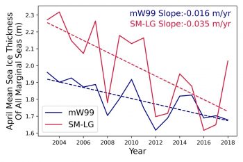
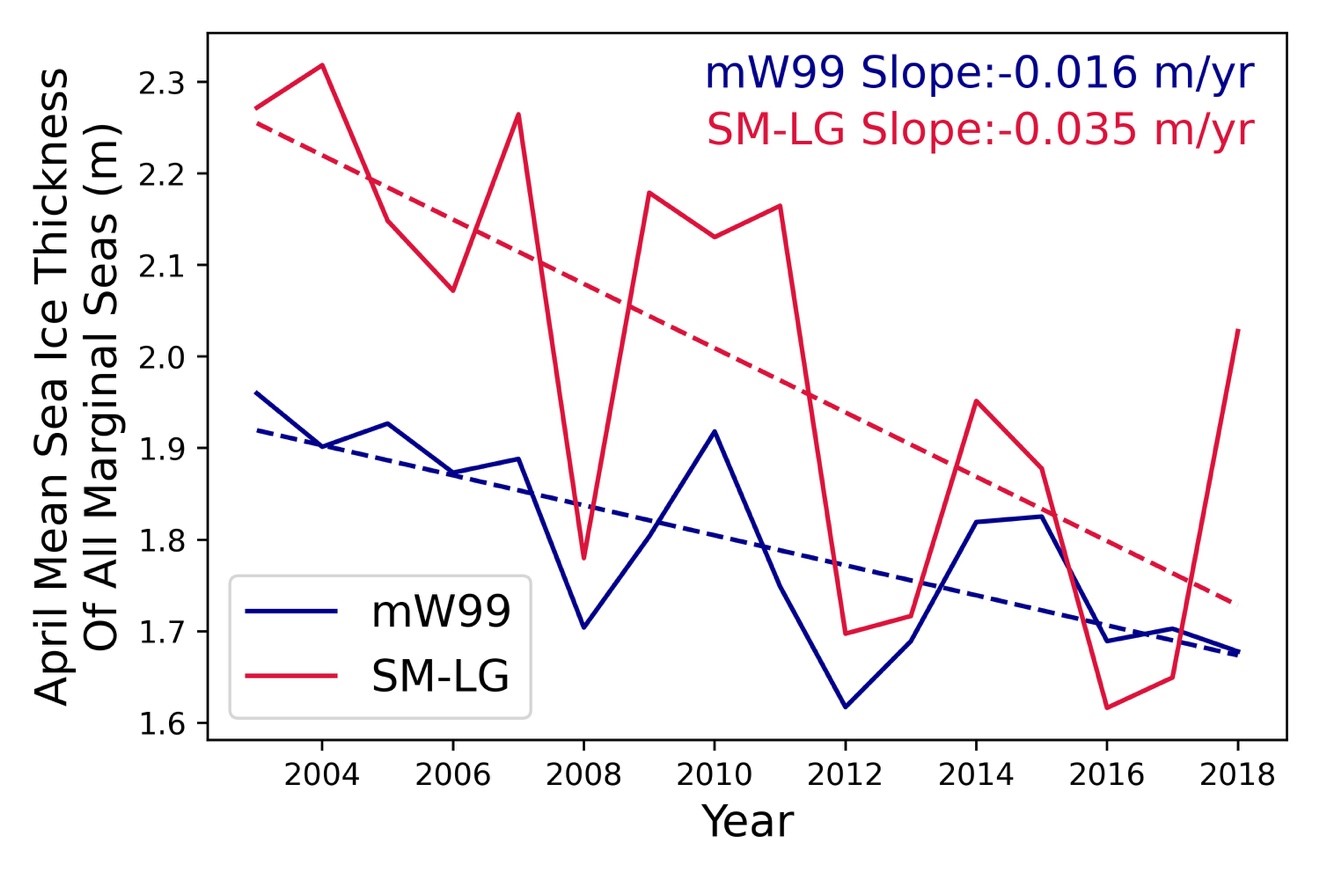
Figure 4. This plot shows average sea ice thickness in the Beaufort, Chukchi, East Siberian, Laptev, Kara, and Barents Seas in April 2004 to 2018 from the Environmental Satellite (Envisat) and CryoSat-2 radar altimeters, processed with the conventional snow product (modified Warren (1999) or mW99) and a new, dynamic snow product (from SnowModel-LG). The rate of decline is more than doubled when processed with SnowModel-LG, as the sea ice thickness inferred from snow cover diminishes.

Credit: R. Mallett, University College London.
High-resolution image

Satellites do not directly measure the thickness of sea ice. They measure the height of the ice surface above the ocean, termed the ice freeboard in the case of radar altimetry, or they measure the height of the ice plus the snow cover, in the case of laser altimetry. To convert these freeboards into total ice thickness requires knowledge of the depth and density of the snow cover atop the ice. Typically, a snow climatology based on snow depth observations collected several decades ago over multiyear ice is used. However, today’s Arctic mostly consists of smoother first-year ice, which tends to have a shallower snow pack than multiyear ice, allowing for deep snow accumulation around ridges. Further, delays in freeze-up and earlier melt onset in today’s warmer climate have reduced the time over which snow can accumulate on the ice. Both factors have resulted in a thinner snowpack than measured 20 years ago.

A new study published in The Cryosphere reveals that when using temporally varying snow depth and density estimates to convert ice freeboard to ice thickness, the ice is thinning at a faster rate in the Arctic marginal seas than previously believed (Figure 4). The time-varying snow depth is from a new data product, the SnowModel-LG, which is soon to be published at the NSIDC Distributed Active Archive Center (DAAC). It is based on coupling a sophisticated snow model with meteorological forcing data from atmospheric reanalysis systems and satellite-derived ice motion vectors. The study found that the rate of decline in ice thickness in the Laptev, Kara, and Chukchi seas was 70, 98 and, 110 percent faster, respectively, compared to previous estimates. As expected, the sea ice thickness variability also increased in response to interannually varying snow depth.

Antarctic notes

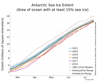
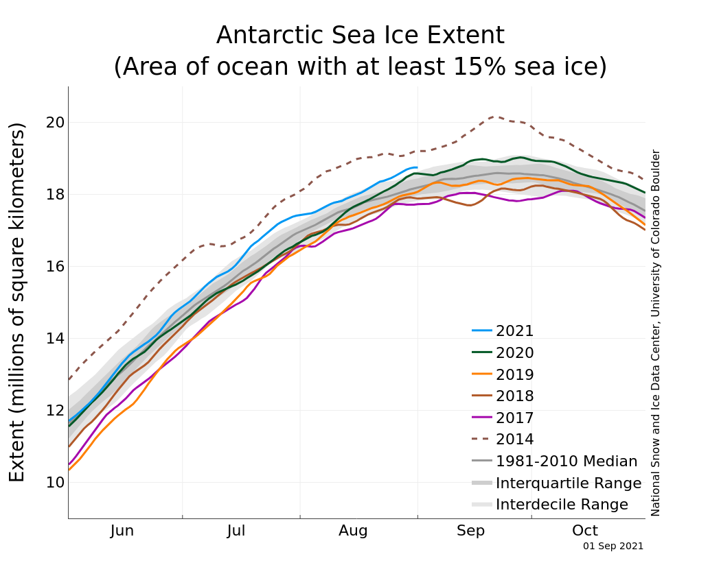
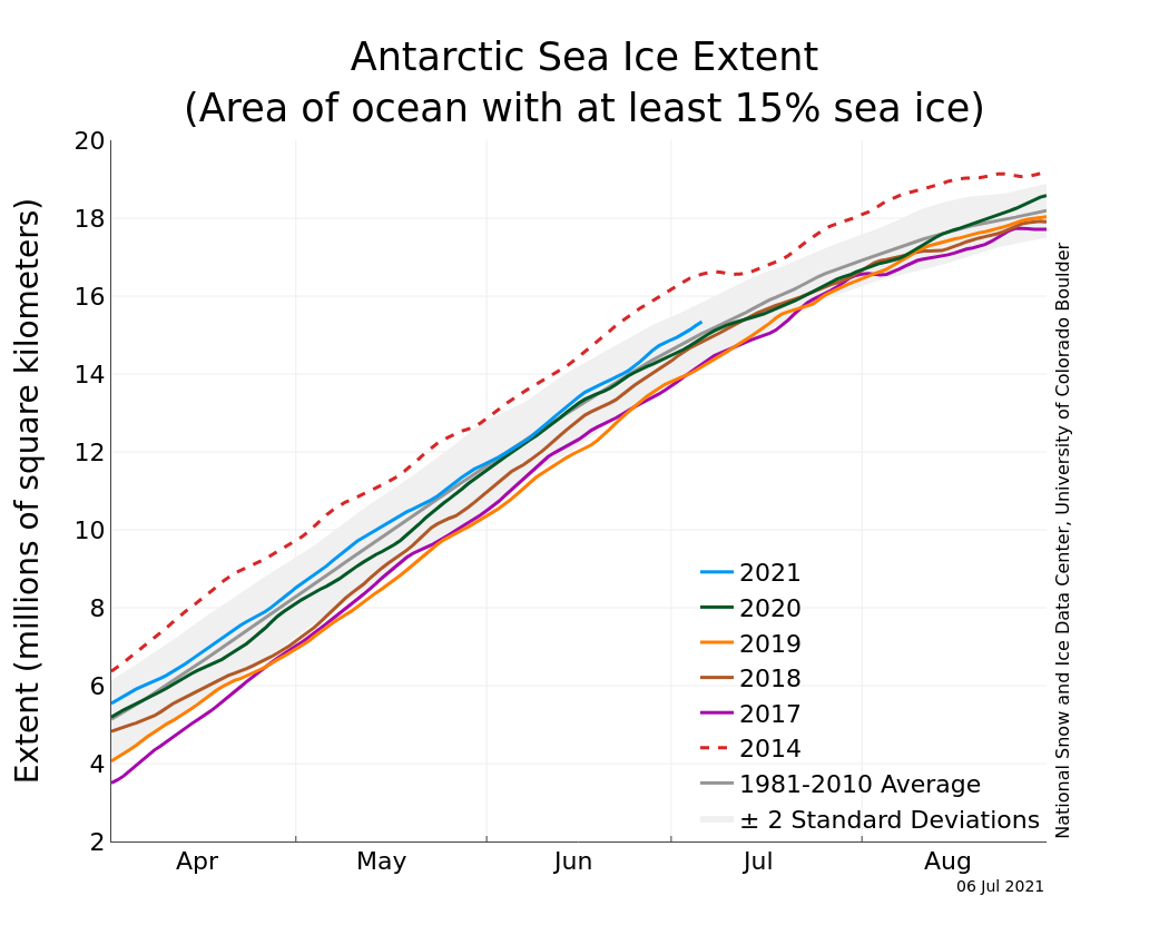
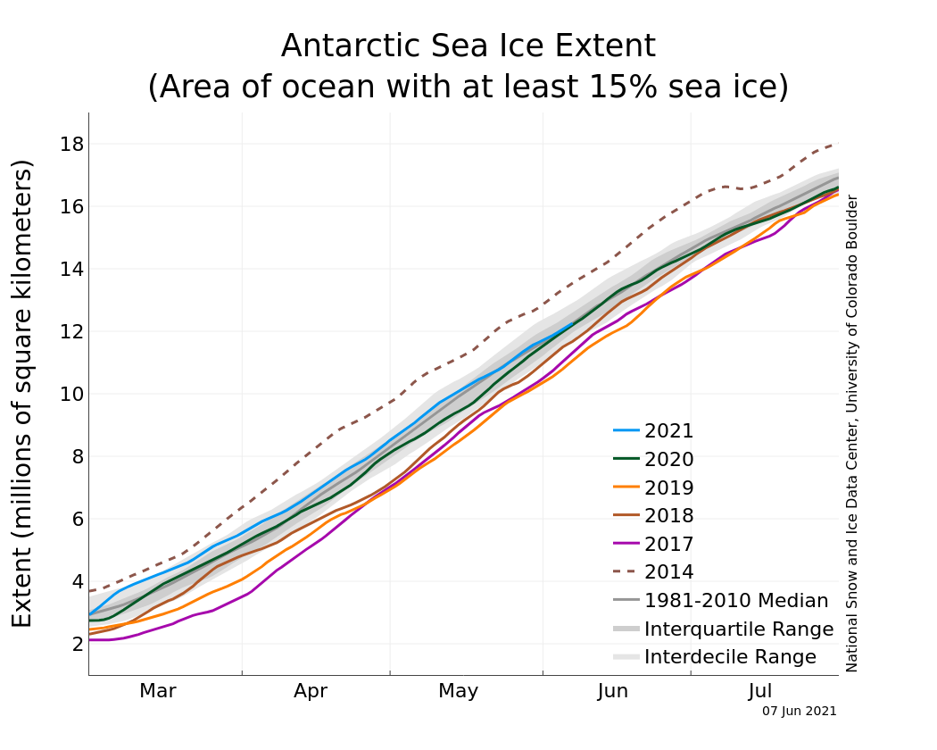
Figure 5a. The graph above shows Antarctic sea ice extent as of June 7, 2021, along with daily ice extent data for four previous years and the record low year. 2021 is shown in blue, 2020 in green, 2019 in orange, 2018 in brown, 2017 in magenta, and 2014 in dashed brown. The 1981 to 2010 median is in dark gray. The gray areas around the median line show the interquartile and interdecile ranges of the data. Sea Ice Index data.

Credit: National Snow and Ice Data Center
High-resolution image

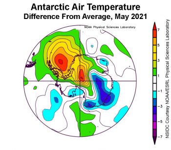
Figure 5b. This plot shows the departure from average air temperature in the Antarctic at the 925 hPa level, in degrees Celsius, for May 2021. Yellows and reds indicate higher than average temperatures; blues and purples indicate lower than average temperatures.

Credit: NSIDC courtesy NOAA Earth System Research Laboratory Physical Sciences Laboratory
High-resolution image

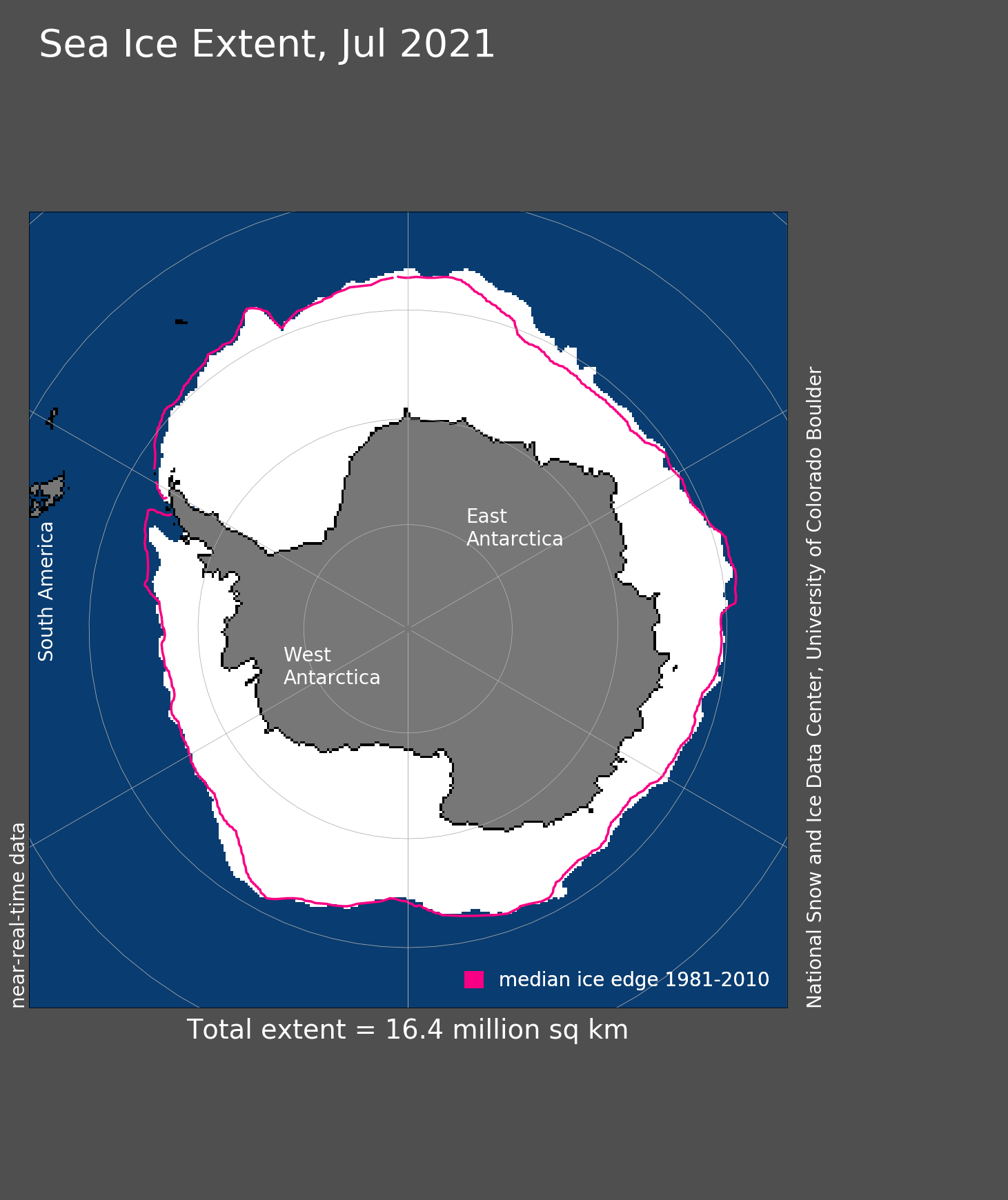
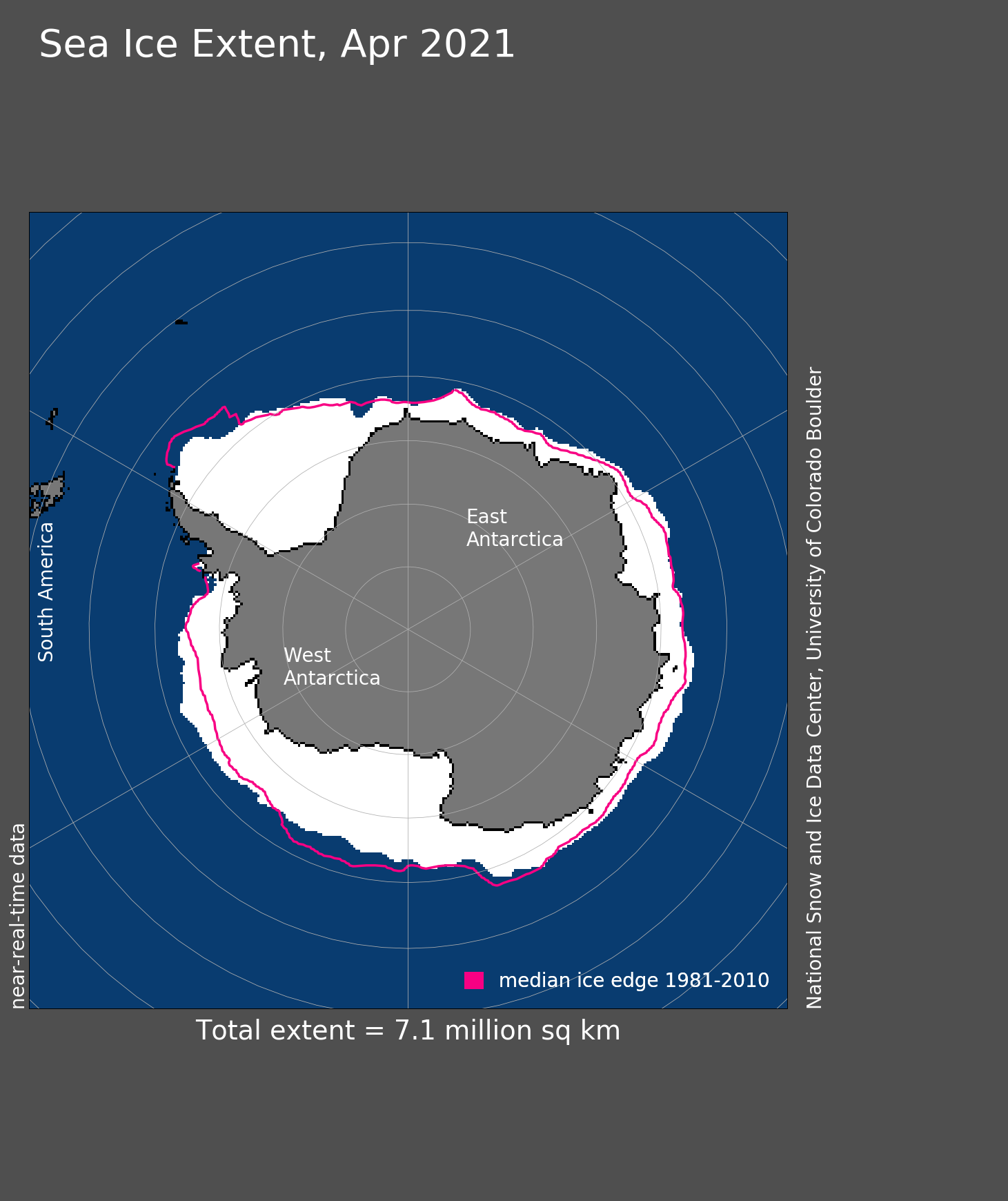
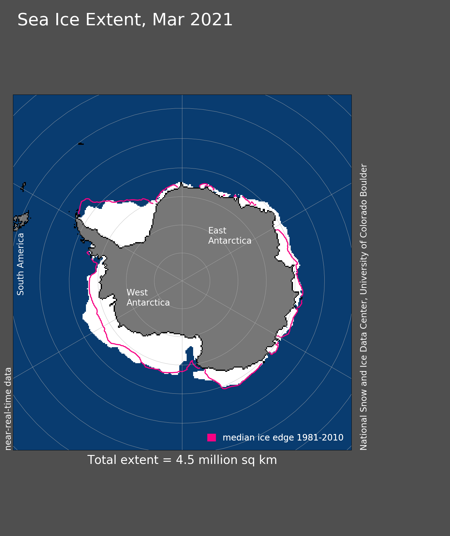
Antarctic sea ice extent grew at a slightly below-average pace in May, moving the overall extent from slightly above average to tracking the 43-year satellite record daily-extent average line (technically, the ‘median’ line) quite closely (Figure 5a). Sea ice extent was below average in the Weddell and Ross Seas, and slightly above average in the Bellingshausen and Amundsen Seas. In keeping with the sea ice trends, air temperatures for the month were well above average over the west-central Weddell Sea, about 7 degrees Celsius (13 degrees Fahrenheit) above average for the month (Figure 5b).

An embayment, or notch, in the ice edge in the eastern Weddell suggests that the processes that create the Maud Rise polynya were active, but at month’s end, the sea ice edge in that area (near 0 degree longitude and 68 degrees S latitude) had not enclosed the potential polynya region.

Further reading

Liston, G. E., P. Itkin, J. Stroeve, M. Tschudi and J. S. Stewart. 2020. A Lagrangian snow-evolution system for sea-ice applications (SnowModel-LG): part I–model description. Journal of Geophysical Research.-Oceans. doi:10.1029/2019JC015913.

Mallett, R. D. C., J. C. Stroeve, M. Tsamados, J. C. Landy, R. Willatt, V. Nandan and G. E. Liston. 2021. Faster decline and higher variability in the sea ice thickness of the marginal Arctic seas. The Cryosphere. doi:10.5194/tc-15-2429-2021.

Martin, J. E. 2021. Recent trends in the waviness of the Northern Hemisphere wintertime polar and subtropical jets. Journal of Geophysical Research-Atmospheres. doi:10.1029/2020JD033668.

Stroeve, J. C., J. Maslanik, M. C. Serreze, I. Rigor and W. Meier. 2011. Sea ice response to an extreme negative phase of the Arctic Oscillation during winter 2009/2010. Geophysical Research Letters. doi: 10.1029/2010GL045662.

Stroeve, J., G. Liston, S. Buzzard, L. Zhou, R. Mallett, A. Barrett, M. Tsamados, M. Tschudi, P. Itkin and J. S. Stewart. 2020. A Lagrangian snow-evolution system for sea ice applications (SnowModel-LG): part II–analyses. Journal of Geophysical Research-Oceans. doi:10.1029/2019JC015900.

Warren, S. G., I. Rigor, N. Untersteiner, V. Radionov, N. Bryazgin, Y. Aleksandrov and R. Colony. 1999. Snow depth on Arctic sea ice. AMS Journey of Climate. doi:10.1175/1520-0442.

The spring decline in Arctic sea ice extent continued at varying rates through the month of April, highlighted by a mid-month pause. Above average air temperatures and low sea level pressure dominated on the Atlantic side of the Arctic, while near average conditions ruled elsewhere.

Overview of conditions

Figure 1. Arctic sea ice extent for April 2021 was 13.84 million square kilometers (5.34 million square miles). The magenta line shows the 1981 to 2010 average extent for that month. Sea Ice Index data. About the data

Credit: National Snow and Ice Data Center
High-resolution image

Arctic sea ice extent averaged for April 2021 was 13.84 million square kilometers (5.34 million square miles). This was 410,000 square kilometers (158,000 square miles) above the record low for the month set in 2019 and 850,000 square kilometers (328,000 square miles) below the 1981 to 2010 average. The average extent for the month ranks sixth lowest in the passive microwave satellite record. Extent was notably low in the Barents and Bering Seas as well as the Labrador Sea. Elsewhere, extent was close to or somewhat below average (Figure 1). The largest ice loss during April was in the Sea of Okhotsk and the Labrador Sea, with smaller losses along the southern edge of the Bering Sea, and in the eastern Barents Sea near the coast of Novaya Zemlya.

Conditions in context

Figure 2a. The graph above shows Arctic sea ice extent as of May 4, 2021, along with daily ice extent data for four previous years and 2012, the record low year. 2021 is shown in blue, 2020 in green, 2019 in orange, 2018 in brown, 2017 in magenta, and 2012 in dashed brown. The 1981 to 2010 median is in dark gray. The gray areas around the median line show the interquartile and interdecile ranges of the data. Sea Ice Index data.

Credit: National Snow and Ice Data Center
High-resolution image

Figure 2b. This plot shows average sea level pressure in the Arctic in millibars from April 14 to 19, 2021. Yellows and reds indicate high air pressure; blues and purples indicate low pressure.

Credit: NSIDC courtesy NOAA Earth System Research Laboratory Physical Sciences Division
High-resolution image

Figure 2c. This plot shows average sea level pressure in the Arctic in millibars for April 2021. Yellows and reds indicate high air pressure; blues and purples indicate low pressure.


Credit: NSIDC courtesy NOAA Earth System Research Laboratory Physical Sciences Division
High-resolution image

Figure 2d. This plot shows the departure from average air temperature in the Arctic at the 925 hPa level, in degrees Celsius, for April 2021. Yellows and reds indicate higher than average temperatures; blues and purples indicate lower than average temperatures.

Credit: NSIDC courtesy NOAA Earth System Research Laboratory Physical Sciences Division
High-resolution image

Sea ice extent remained below the tenth percentile range throughout the month of April. However, rate of decline was variable. Notably, the decline paused, and extent even slightly increased between April 14 and April 19 (Figure 2a). This was largely because of an increase in sea ice in the northern Barents Sea, particularly off the northwest coast of Novaya Zemlya.

This temporary ice expansion appears to have been primarily driven by low sea level pressure centered over the Laptev Sea (Figure 2b). This led to winds from the north in the northern Barents Sea, pushing ice southward. The sea level pressure pattern for the full month featured low pressure centered in the Barents Sea, north of the Scandinavian coast (Figure 2c); bringing warm winds from the south and above average monthly temperatures in the region. Elsewhere in the Arctic, conditions were more moderate with 925 mb temperatures 1 to 3 degrees Celsius (2 to 5 degrees Fahrenheit) above average and weak high pressure (Figure 2d).

April 2021 compared to previous years

Figure 3. Monthly April ice extent for 1979 to 2021 shows a decline of 2.6 percent per decade.

Credit: National Snow and Ice Data Center
High-resolution image

Through 2021, the linear rate of decline for April sea ice extent, relative to the 1981 to 2010 average extent, is 2.6 percent per decade (Figure 3). This corresponds to 38,600 square kilometers (14,900 square miles) per year, about the size of the US states of New Hampshire and Connecticut combined. The cumulative April ice loss over the 43-year satellite record is 1.62 million square kilometers (625,000 square miles), based on the difference in linear trend values in 2021 and 1979, which is equivalent in size to 2.3 times the size of the state of Texas.

Sea ice age update

Figure 4. This figure compares sea ice age between March 12 to 18 for the years 1985 (a) and 2021 (b). The bottom graph (c) shows a time series from 1985 to 2021 of percent ice coverage of the Arctic Ocean domain. The Arctic Ocean domain is depicted in the inset map with purple shading. 

Credit: M. Tschudi, University of Colorado, and W. Meier and J.S. Stewart, National Snow and Ice Data Center/Image by W. Meier
High-resolution image

The sea ice continues to be far younger, and thus thinner, than in the 1980s. There is little change in the age distribution from last year. At the end of the ice growth season in mid-March, 73.3 percent of the Arctic Ocean domain was covered by first-year ice, while 3.5 percent was covered by ice 4+ years old. This compares to 70.6 percent and 4.4 percent respectively in March 2020. In March 1985, near the beginning of the ice age record, the Arctic Ocean region was comprised of nearly equal amounts of first-year ice (39.3 percent) and 4+ year-old ice (30.6 percent).

In 2021, the extremely high sea level pressure in February over the central Arctic Ocean produced a strong Beaufort Gyre sea ice circulation, as noted in our March post. This pushed a substantial amount of ice, including older ice, onto the northern Alaskan and Canadian coast in the Beaufort Sea. Some of this ice has now moved north and west into the Chukchi Sea–an isolated patch of older ice amidst first-year ice. This will bear watching through the summer to see the fate of that older ice.

Antarctica

Figure 5: Antarctic sea ice extent for April 2021 was 7.08 million square kilometers (2.73million square miles). The magenta line shows the 1981 to 2010 average extent for that month. Sea Ice Index data. About the data

Credit: National Snow and Ice Data Center
High-resolution image

In the Antarctic, autumn is now in full swing, but ice growth has been somewhat sluggish through the month. At the beginning of the month, extent was between the seventy-fifth and ninetieth percentile range of the 1981 to 2010 climatology. By the end of the month, extent was within the inner quartile range and just above the median.

Antarctic extent for April 2021 was 7.08 million square kilometers (2.73 million square miles), 230,000 square kilometers (88,800 square miles) above the 1981 to 2010 average (Figure 5). Extent was low in the northwestern Weddell Sea region and northern Ross Sea, and both areas had temperatures 3 to 8 degrees Celsius (5 to 14 degrees Fahrenheit) above the reference period. Sea ice extent was generally above average elsewhere, particularly in the Amundsen Sea, where rather cool conditions prevailed for April, at 1 to 3 degrees Celsius (2 to 5 degrees Fahrenheit) below average.

Seasonal predictability of Arctic sea ice from ocean heat transport

Figure 6. This figure shows correlations between ocean heat transport through the Bering strait and sea ice concentration in the Arctic Ocean. Heat transport anomalies in May are compared to June (left) and July (right) sea ice concentration anomalies. Red areas show regions of the Arctic Ocean where Pacific Ocean heat has the strongest influence on sea ice conditions. Significant correlations at the 95 percent significance level are outlined in black. Regions where the interannual variability in monthly sea ice concentration is larger than 10 percent are outlined in green. An anomaly refers to the deviation of ocean heat transports and sea ice concentrations from their linear trends.


Credit: image adapted from Lenetsky et al. (2021).
High-resolution image

As the Arctic summer nears, the Sea Ice Prediction Network team, which includes NSIDC scientists, is gearing up for another year of the Sea Ice Outlook. Participants in the Outlook and other researchers are investigating ways to better understand and improve seasonal predictability of Arctic September sea ice extent. One factor in sea ice predictability is ocean heat.

A recent study led by University of Colorado master’s student Jed Lenetsky, in collaboration with researchers at McGill University and the Massachusetts Institute of Technology, examined the influence of Pacific Ocean heat on sea ice conditions. Results show that Pacific Ocean heat entering the Arctic Ocean through the Bering Strait has the largest influence on sea ice conditions in the spring and early summer in the Chukchi Sea, fostering early opening of the pack ice and triggering the ice-albedo feedback (Figure 6). From August through October, the summer stratification of the Chukchi Sea reduces the influence of Pacific Ocean heat on sea ice conditions. At the same time, other processes, such as ocean heat uptake and wind-induced sea ice drift, become the dominant drivers of sea ice variability in the region. The influence of the Bering Strait heat transport re-emerges in November as a factor in the timing of freeze onset. These results have important implications for seasonal sea ice prediction in the Chukchi Sea, as predictions using Pacific Ocean heat are more skillful than predictions using more commonly used parameters such as sea ice concentration and sea ice thickness.

Further reading

Lenetsky, J. E., B. Tremblay, C. Brunette, and G. Meneghello. 2021. Subseasonal predictability of Arctic Ocean sea ice conditions: Bering Strait and Ekman-driven ocean heat transport.  J. Climate. doi:10.1175/JCLI-D-20-0544.1.

The seasonal maximum extent of Arctic sea ice has passed, and with the passing of the vernal equinox, the sun has risen at the north pole. While there are plenty of cold days ahead, the long polar night is over. Arctic sea ice extent averaged for March 2021 was the ninth lowest in the satellite record. With little ice in the Gulf of St. Lawrence, harp seal pups are struggling. At month’s end, Antarctic sea ice extent was slightly above average.

Overview of conditions

Figure 1. Arctic sea ice extent for March 2021 was 14.64 million square kilometers (5.65 million square miles). The magenta line shows the 1981 to 2010 average extent for that month. Sea Ice Index data. About the data

Credit: National Snow and Ice Data Center
High-resolution image

Arctic sea ice extent averaged for March 2021 was 14.64 million square kilometers (5.65 million square miles). This was 350,000 square kilometers (135,000 square miles) above the record minimum set in 2017 and 790,000 square kilometers (305,000 square miles) below the 1981 to 2010 average. The average extent ranks ninth lowest in the satellite record, which began in 1979. Regionally, extent at the end of the month was below average on the Pacific side in the Bering sea and on the Atlantic side in the northern Barents Sea and well south of the Arctic in the Gulf of St. Lawrence. Elsewhere, extent was close to the average, though generally somewhat lower. Ice loss during March was primarily in the Sea of Okhotsk, the southern edge of the Bering Sea, east of Svalbard, and in the northern part of the East Greenland Sea. The ice edge expanded in the southern part of the East Greenland Sea and to the north of Svalbard.

Conditions in context

Figure 2a. The graph above shows Arctic sea ice extent as of April 5, 2021, along with daily ice extent data for four previous years and the 2012 record low. 2020 to 2021 is shown in blue, 2019 to 2020 in green, 2018 to 2019 in orange, 2017 to 2018 in brown, 2016 to 2017 in magenta, and 2011 to 2012 in dashed brown. The 1981 to 2010 median is in dark gray. The gray areas around the median line show the interquartile and interdecile ranges of the data. Sea Ice Index data.

Credit: National Snow and Ice Data Center
High-resolution image

Figure 2b. This plot shows the departure from average air temperature in the Arctic at the 925 hPa level, in degrees Celsius, for March 2021. Yellows and reds indicate higher than average temperatures; blues and purples indicate lower than average temperatures.

Credit: NSIDC courtesy NOAA Earth System Research Laboratory Physical Sciences Division
High-resolution image

Figure 2c. This plot shows average sea level pressure in the Arctic in millibars March 2021. Yellows and reds indicate high air pressure; blues and purples indicate low pressure.

Credit: NSIDC courtesy NOAA Earth System Research Laboratory Physical Sciences Division
High-resolution image

During March, sea ice extent tracked well below average, but as noted in our previous post, the seasonal maximum in extent, reached on March 21, one day after the vernal equinox, was only the seventh lowest in the passive microwave satellite record. Since ice extent in March increases through the first part of the month and then decreases thereafter, the daily average growth rate is not a very meaningful statistic.

Air temperatures at the 925 mb level (about 2,500 feet above sea level) in March were up to 5 degrees Celsius (9 degrees Fahrenheit) below average across northern Eurasia and extending east over Alaska. Temperatures were 1 to 3 degrees Celsius (2 to 5 degrees) Celsius above average over the Atlantic side of the Arctic, with a tongue of above-average temperatures extending into the Beaufort Sea (Figure 2b). The associated atmospheric circulation for March features low pressure over the northern North Atlantic, with the lowest pressure focused over the Barents Sea (Figure 2c). After remaining in a fairly persistent negative phase for much of the past winter, the Arctic Oscillation index in March was mostly positive, but with large fluctuations.

March 2021 compared to previous years

Figure 3. Monthly March ice extent for 1979 to 2021 shows a decline of 2.6 percent per decade.

Credit: National Snow and Ice Data Center
High-resolution image

Through 2021, the linear rate of decline for March sea ice extent, relative to the 1981 to 2010 average extent, is 2.6 percent per decade, which corresponds to 39,700 square kilometers (15,300 square miles) per year, about the size of the US states of Maryland and Delaware combined or the country of Switzerland. The cumulative March ice loss over the 43-year satellite record is 1.67 million square kilometers (645,000 square miles), based on the difference in linear trend values in 2021 and 1979, which is equivalent in size to the state of Alaska.

Troubles in the Gulf of St. Lawrence

Figure 4. A harp seal pup rests on sea ice. Harp seal pups are born with long white fur that helps them absorb sunlight and stay warm while they develop blubber. Pups shed their white fur after about three to four weeks old.

Credit: Flickr/laika_ac
High-resolution image

This winter ice extent was far below average in the Gulf of St. Lawrence, which is an outlet for the US Great Lakes located northeast of New Brunswick. The unusually low sea ice extent is leading to the death of many harp seal pups. In December, harp seals arrive at the Gulf of St. Lawrence from the Canadian Arctic and Greenland, and then give birth to pups under snow on the ice cover.  With so little sea ice, many pups were forced to cluster on shore where they are vulnerable to predators, leading to high pup mortality. It is widely viewed that with continued warming and loss of sea ice, harp seal populations will decline.

Antarctic sea ice on the rise

Figure 5. Antarctic sea ice extent for March 2021 was 4.45 million square kilometers (1.72 million square miles). The magenta line shows the 1981 to 2010 average extent for that month. Sea Ice Index data. About the data

Credit: National Snow and Ice Data Center
High-resolution image

After reaching its seasonal minimum extent on February 21, Antarctic sea ice extent climbed rapidly, passing the long-term average daily extent on March 1. The rate of growth was very rapid between February 25 and March 8, expanding by over one million square kilometers (386,000 square miles) in the 12-day period. This is the fastest expansion in the four-decade record of sea ice extent for this time of year, and was caused by a rapid refreezing of the western Amundsen Sea and eastern Ross Sea areas. Since early March, growth has slowed to a more typical, slightly below-average pace. The Amundsen and eastern Ross Seas remain well above the average extent for the season. Sea ice extent in the Bellingshausen Sea and Weddell Sea are slightly below average. At the end of the month, Antarctic ice extent neared 5.5 million square kilometers (2.1 million square miles).