Descriptions of and differences between the NASA Team and Bootstrap algorithms
NSIDC currently archives passive microwave sea ice concentration products based on two algorithms: the NASA Team algorithm and the Bootstrap algorithm. Both algorithms were developed by researchers at the NASA Goddard Space Flight Center in the 1980s. Provided below are two short summaries of the algorithms, an overview of the differences between them, and relevant references.
NASA Team algorithm
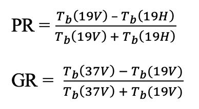
The NASA Team algorithm calculates sea ice concentration by comparing the ratios between three vertically (V) and horizontally (H) brightness temperature (Tb) channels: 19V, 19H, and 37V. Specifically, the algorithm relies on two Tb ratios: the polarization ratio (PR) and the spectral gradient ratio (GR), defined below:
PR and GR values tend to cluster around three values (see figure below), each of which corresponds to a different surface type: a water (ice-free) surface or one of two sea ice surface types. In the Arctic, the two ice types correspond to first-year ice (FYI), i.e. ice that has formed since the previous summer, and multiyear ice (MYI), i.e. ice that has survived at least one summer melt season. In the Antarctic, there is not clear discrimination between first-year and multi-year ice, so the two types are simply described as Type A and Type B. Based on these three Tb clusters, constant coefficients, called “tie-points”, are derived to represent 100% concentrations of each surface type. These form the vertices of a triangle (see figure below). PR and GR values that fall between these vertices represent a mixture of surface types. The NASA Team algorithm relies on nine tie-points, each representing a combination of surface type (ice-free ocean, first-year sea ice, and multiyear sea ice) and channel (19H, 19V, and 37V) used in the algorithm. There are unique sets of tie-points for each hemisphere and each sensor used in the data product. Adjustments in tie-points between sensors is done via inter-calibration using sensor overlap periods. See Cavalieri et al. (1997) for a list of tie points.
Figure 1: PR vs GR scatterplot

Lastly, the NASA Team algorithm applies a weather filter to remove spurious sea ice concentration estimates (see figure above). This weather filter is based on the GR for the 37V and 19V channels and incorporates an additional GR using the 22V and 19V channels, as shown below and as described in Table 1:
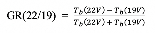
Table 1. Weather filter criteria
| SSMR-derived data | GR(37/19) > 0.07 |
|---|---|
| SSMI-derived data | GR(37/19) > 0.050 and/or GR(22/19) > 0.045 |
| SSMIS-derived data | GR(37/19) > 0.053 |
Sea ice concentrations are set to 0 whenever GR calculations meet the criteria outlined in Table 1. In practice, the GR threshold tends to eliminate any ice with concentrations below 15%.
The NASA Team algorithm is least accurate in regions where there is surface melt or thin ice. It is not designed to provide ice concentrations over fresh-water.
Bootstrap algorithm
The Bootstrap algorithm uses brightness temperature (Tb) observations from the 37H, 37V and 19V channels to estimate sea ice concentration. Scatterplots of Tb observations from two channels show non-linear clusters of data. For example, there are clusters of Tb values for open water and 100% ice covered regions (see the figure below for an example). Sea ice concentrations between 0 and 100% can thus derived by determining 1) the equation of the line (AD) for the cluster representing 100% ice and the value of the cluster (O) representing open water, and 2) matching Tb values along a line between AD and 0 to a corresponding sea ice concentration via linear interpolation. Within the ice pack (away from the ice edge), scatterplots of the two 37H and 37V are used; this region is delineated by points above the AD-5 line in the figure below. Near the ice edge (values below the AD-5 line in the figure below), the 37V and 19V channels are used to derive the concentration values, because the 37V and 19V combination is more sensitive to the ice-water boundary. The Bootstrap algorithm utilizes tie points to identify clusters of Tb values; these tie points change daily and between hemispheres (Northern / Southern), based on the properties of each day’s Tb fields. See Comiso (1995) for a description of how tie points are derived.
Figure 2: Scatterplots of Tb observations from two channels show non-linear clusters of data

The Bootstrap algorithm uses a filter to identify areas where weather-related effects might have affected sea ice concentration estimates. This weather filter is also based on interpolation between clusters of known Tb observations and incorporates observations from an additional channel: 22V. The figure below demonstrates how the V19/V22-V19 and V19/V37 scatterplots can be used to identify areas of spurious estimates.
Figure 3: 22V-19V vs 19V

Sea ice concentration maps generated by the Bootstrap algorithm generally have a well identified marginal ice zone and very high sea ice concentration values in the inner pack. However, the actual concentration gradient near the sea ice edge may be higher than what the algorithm predicts. This is partly due to changes in emissivity between the ice edge (where first-year ice predominates) and the inner pack (where multiyear ice predominates) and partly because sensors tend to smear the data when the satellite passes a boundary of two contrasting surfaces (due to limited spatial resolution). Like the NASA Team algorithm, the Bootstrap algorithm is least accurate in regions where there is surface melt or thin ice.
Differences between the algorithms
The main differences between the NASA Team and Bootstrap algorithms are described below.
Table 2. Main differences between NASA Team and Bootstrap algorithms
NASA Team | Bootstrap | |
|---|---|---|
Channels used to derive sea ice concentration | 19V, 19H, 37V | 19V, 37H, 37V |
Methodology | Algorithm is based on ratios of brightness temperatures (Tb) using coefficients (tie points) for pure surface types (open ocean and 100% concentration sea ice). | Algorithm is based on scatterplot interpolation between brightness temperatures (Tb) observation clusters from pure ice types (e.g. open ocean and 100% concentration sea ice). |
Tie points | Unique tie points for each hemisphere | Tie points change by date (dynamic) and hemisphere |
Weather filter | Filter is based on the 37V and 19V Tb ratios for all SMMR-derived data. SSMI- and SSMIS-derived data also use the 22V and 19V ratios. | Filter is based on scatterplots of 19V vs 22V-19V Tb and 19V vs 37V Tb (Figure 3). |
Limitations | Algorithm has difficulty distinguishing ice types (multi-year / first year) during the spring melt. Algorithm underestimates thin ice. | Open water estimates may include grease ice / nilas / new ice. |
| Strengths | Not sensitive to changes in surface temperature. | Less sensitive to thin ice and layering of snow and ice. |
| Weaknesses | Sensitive to thin ice and layering of snow and ice. | Sensitive to changes in surface temperature. |
| Accuracy | Errors are <5% for high-concentration winter ice away from the ice edge. | |
| Primary Citations | Cavalieri, D. J., C. L. Parkinson, P. Gloersen, & H. J. Zwally. 1997. Arctic and Antarctic Sea Ice Concentrations from Multichannel Passive-Microwave Satellite Data Sets: October 1978-September 1995 - User's Guide. NASA Technical Memorandum 104647. Goddard Space Flight Center, Greenbelt, MD 20771. 17 pg. Available from: https://ntrs.nasa.gov/search.jsp?R=19980076134 Cavalieri, D. J., P. Gloersen, and W. J. Campbell. 1984. Determination of sea ice parameters with the Nimbus 7 SMMR. J. Geophys. Res., 89, 5355-5369. https://doi.org/10.1029/JD089iD04p05355 | Comiso, J. C. 1995. SSM/I Concentrations Using the Bootstrap Algorithm. NASA Reference Publication 1380. 40 pg. Available from: https://www.geobotany.uaf.edu/library/pubs/ComisoJC1995_nasa_1380_53.pdf Comiso, J. C., & F. Nishio. 2008. Trends in the Sea Ice Cover Using Enhanced and Compatible AMSR-E, SSM/I, and SMMR Data. Journal of Geophysical Research, 113, C02S07. https://doi.org/10.1029/2007JC004257 |
NSIDC data sets that use each algorithm
References
For information on the accuracy of each algorithm and comparisons between the two, see the following references:
Andersen, S., Tonboe, R., Kaleschke, L., Heygster, G., & Pedersen, L. T. (2007). Intercomparison of passive microwave sea ice concentration retrievals over the high-concentration Arctic sea ice. Journal of Geophysical Research, 112(C8), C08004. https://doi.org/10.1029/2006JC003543
Cavalieri, D. J., P. Gloersen, and W. J. Campbell. 1984. Determination of sea ice parameters with the Nimbus 7 SMMR. J. Geophys. Res., 89, 5355-5369. https://doi.org/10.1029/JD089iD04p05355
Cavalieri, D. J., C. L. Parkinson, P. Gloersen, & H. J. Zwally. 1997. Arctic and Antarctic Sea Ice Concentrations from Multichannel Passive-Microwave Satellite Data Sets: October 1978-September 1995 - User's Guide. NASA Technical Memorandum 104647. Goddard Space Flight Center, Greenbelt, MD 20771. 17 pg. Available from: https://ntrs.nasa.gov/search.jsp?R=19980076134
Comiso, J. C. 1995. SSM/I Concentrations Using the Bootstrap Algorithm. NASA Reference Publication 1380. 40 pg. Available from: https://www.geobotany.uaf.edu/library/pubs/ComisoJC1995_nasa_1380_53.pdf
Comiso, J. C., Cavalieri, D. J., Parkinson, C. L., & Gloersen, P. (1997). Passive microwave algorithms for sea ice concentration: A comparison of two techniques. Remote Sensing of Environment, 60(3), 357–384. https://doi.org/10.1016/S0034-4257(96)00220-9
Comiso, J. C., & F. Nishio. 2008. Trends in the Sea Ice Cover Using Enhanced and Compatible AMSR-E, SSM/I, and SMMR Data. Journal of Geophysical Research, 113, C02S07. https://doi.org/10.1029/2007JC004257
Ivanova, N., Pedersen, L. T., Tonboe, R. T., Kern, S., Heygster, G., Lavergne, T., Sørensen, A., Saldo, R., Dybkjær, G., Brucker, L., & Shokr, M. (2015). Inter-comparison and evaluation of sea ice algorithms: Towards further identification of challenges and optimal approach using passive microwave observations. The Cryosphere, 9(5), 1797–1817. https://doi.org/10.5194/tc-9-1797-2015
Kern, S., Lavergne, T., Notz, D., Pedersen, L. T., & Tonboe, R. T. (2020). Satellite passive microwave sea-ice concentration data set intercomparison for arctic summer conditions [Preprint]. Sea ice/Remote Sensing. https://doi.org/10.5194/tc-2020-35
Kern, S., Lavergne, T., Notz, D., Pedersen, L. T., Tonboe, R. T., Saldo, R., & Sørensen, A. M. (2019). Satellite passive microwave sea-ice concentration data set intercomparison: Closed ice and ship-based observations. The Cryosphere, 13(12), 3261–3307. https://doi.org/10.5194/tc-13-3261-2019
Meier, W. N. (2005). Comparison of passive microwave ice concentration algorithm retrievals with AVHRR imagery in arctic peripheral seas. IEEE Transactions on Geoscience and Remote Sensing, 43(6), 1324–1337. https://doi.org/10.1109/TGRS.2005.846151