The fast pace of ice loss observed in the beginning of July continued through the third week of July, after which the ice loss rates slowed dramatically. Above-average air temperatures and extensive melt pond development helped to keep the overall sea ice extent at record low levels, however, leading to a new record low for the month of July. Toward the end of the month, a strong low pressure system moved into the ice in the Beaufort Sea region. Antarctic sea ice extent remains below average levels as it climbs towards its seasonal maximum, which is typically reached in early October.
Overview of conditions
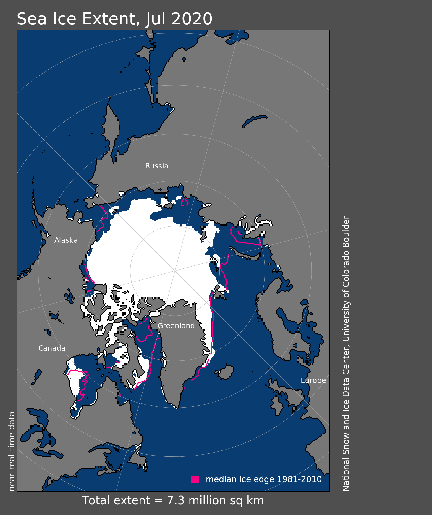
Figure 1. Arctic sea ice extent for July 2020 was 7.28 million square kilometers (2.81 million square miles). The magenta line shows the 1981 to 2010 average extent for that month. Sea Ice Index data. About the data
Credit: National Snow and Ice Data Center
High-resolution image
Sea ice extent averaged for July 2020 was 7.28 million square kilometers (2.81 million square miles), the lowest extent in the satellite record for the month. This was 2.19 million square kilometers (846,000 square miles) below the 1981 to 2010 July average and 310,000 square kilometers (120,000 square miles) below the previous record low mark for July set in 2019.
Arctic sea ice extent continued to track at record low levels through the end of July, dominated by extensive open water in the East Siberian, Laptev, and Kara Seas. As of July 31, sea ice was tracking 187,000 square kilometers (72,200 square miles) below 2019, which held the previous record for least amount of sea ice on that date, and 396,000 square kilometers (153,000 square miles) below 2012, the year of the record low. The ice edge was further north than average everywhere except the southeastern Beaufort Sea, the Canadian Archipelago and the East Greenland Sea.
Because of the unusually early retreat of sea ice on the Siberian side of the Arctic, the Northern Sea Route appears ice-free in the satellite passive microwave data record in the second half of the month. This is the earliest in the year that the route has been free of ice, according to this data record. However, the MASIE sea ice product, which relies on data from several satellite sources and is provided through collaboration with the U.S. National Ice Center, shows some ice remaining south of Severnaya Zemlya. While ice chart data tend to be conservative, it appears that the route likely will be open for the next two to three months.
While ice retreated at a fast pace through the first three weeks of July, it started to slow around July 23 as the retreating ice edge approached areas of higher-concentration ice that does not melt out as readily. Nevertheless, July 2020 set a new record low sea ice extent over the satellite time-period.
Conditions in context

Figure 2a. The graph above shows Arctic sea ice extent as of August 3, 2020, along with daily ice extent data for four previous years and the record low year. 2020 is shown in blue, 2019 in green, 2018 in orange, 2017 in brown, 2016 in purple, and 2012 in dashed red. The 1981 to 2010 median is in dark gray. The gray areas around the median line show the interquartile and interdecile ranges of the data. Sea Ice Index data.
Credit: National Snow and Ice Data Center
High-resolution image
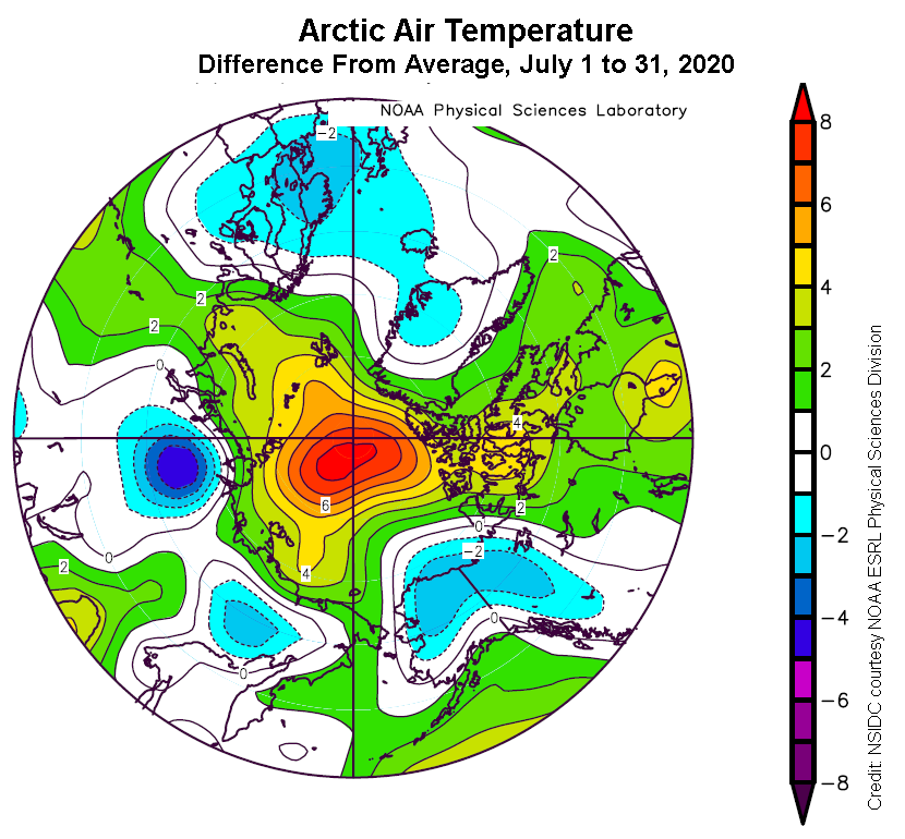
Figure 2b. This plot shows the departure from average air temperature in the Arctic at the 925 hPa level, in degrees Celsius, from July 1 to 31, 2020. Yellows and reds indicate higher than average temperatures; blues and purples indicate lower than average temperatures.
Credit: NSIDC courtesy NOAA Earth System Research Laboratory Physical Sciences Division
High-resolution image
Through the month, sea ice declined by an average of 116,000 square kilometers (44,800 square miles) per day, faster than the 1981 to 2010 average of 86,800 square kilometers (33,500 square miles) per day. This corresponds to a total loss of 3.59 million square kilometers (1.39 million square miles) of ice extent during July 2020.
The average near-surface air temperatures at the 925 hPa level (about 2,500 feet above sea level) for July was up to 8 degrees Celsius (14 degrees Fahrenheit) above average over the central Arctic Ocean centered near the pole. Coastal regions experienced temperatures between 2 and 4 degrees Celsius (4 to 7 degrees Fahrenheit) above average. Above-average air temperatures also stretched further south through Baffin Bay and Davis Strait. The exception was the southern Beaufort Sea which was 1 to 2 degrees Celsius (2 to 4 degrees Fahrenheit) cooler than average. The warm conditions of the first half of July continued through the third week of July. This temperature pattern reflects unusually high sea level pressure over the Laptev, East Siberian, and Chukchi Seas and Greenland, coupled with unusually low sea level pressure over the Central Arctic Ocean and over the North Atlantic Ocean, centered north of Iceland. This pattern has brought warm air over Siberia, extending to the coastal regions while allowing cold Arctic air to spill out into Russia.
July 2020 compared to previous years
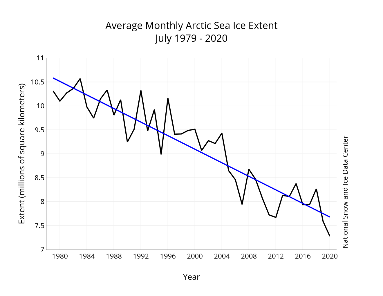
Figure 3. Monthly July sea ice extent for 1979 to 2020 shows a decline of 7.48 percent per decade.
Credit: National Snow and Ice Data Center
High-resolution image
Including 2020, the linear rate of decline of July sea ice extent is 7.48 percent per decade, or 70,800 square kilometers (27,300 square miles) per year. This corresponds to about the size of the state of North Dakota. Over the 42-year satellite record, the Arctic has lost about 2.90 million square kilometers (1.12 million square miles) of ice in July, based on the difference in linear trend values in 2020 and 1979. This is comparable to about the size of the states of Alaska, Texas, and California combined.
Cyclone in the Beaufort Sea

Figure 4. This figure shows four images that depict an Arctic cyclone from July 27 to 30, 2020. Image a in the upper left-hand corner is a NASA Moderate Resolution Imaging Spectroradiometer (MODIS) composite image from NASA Worldview that shows the cyclone in Beaufort Sea region on July 29. Image b in the upper right-hand corner shows a Japan Aerospace Exploration Agency (JAXA) Advanced Microwave Scanning Radiometer 2 (AMSR2) sea ice concentration map from the University of Bremen for July 29 that shows the same area as in a. Image c in the lower left-hand corner shows the surface pressure from Climate Reanalyzer for July 29. Image d in the lower right-hand corner shows the wind speed for July 29 from Climate Reanalyzer.
Credit: National Snow and Ice Data Center
High-resolution image
A strong, but not exceptional, cyclone with a minimum sea level pressure of 975 hPa on July 28 entered the Beaufort Sea from Alaska in late July. Winds along the sea ice edge reached about 12 meters per second (23 knots). While the cyclone gradually weakened through the next few days, it appears to have forced some ice divergence within the East Siberian Sea such that the ice edge expanded slightly southwards. The storm temporarily caused atmospheric and surface effects on the passive microwave signal due to emission from the thick clouds and changes in the snow and sea ice surface properties (Figure 4). This is illustrated in the sea ice concentration fields (Figure 4b), where concentrations are reduced, particularly in the “eye” of the storm—the small circular region near the center of the image north of Utqiagvik that has much lower concentration ( the green color corresponds to about 50 percent concentration). The spiral circulation pattern is also quite clear in the Bremen sea ice concentrations, which is an atmospheric and surface effect due to the storm, not a real pattern of concentration. However, early indications are that some spreading of the ice pack occurred, and this may permit somewhat faster sea ice decline in the coming weeks in this area. A similar storm in 2012—the record low sea ice extent year—led to effects that augmented the decline in that year.
Melt onset and melt ponds
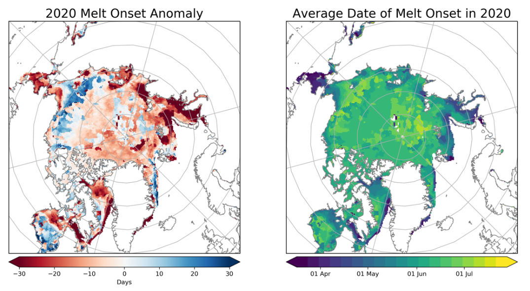
Figure 5a. This figure shows the melt onset anomaly (left) and mean melt onset dates (right) for 2020. Anomaly is computed relative to the 1981 to 2010 average. Melt detection is based on passive microwave brightness temperatures following the algorithm described in Markus et. al. 2009.
Credit: Linette Boisvert and Jeffrey Miller, NASA Goddard Space Flight Center
High-resolution image
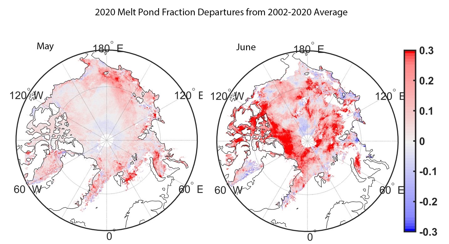
Figure 5b. This figure shows melt pond fractional area anomalies for May (left) and June (right). Red colors show more extensive melt ponds relative to the 2002 to 2020 average, whereas blue colors show fewer melt ponds than average.
Credit: Sanggyun Lee, University College London
High-resolution image
The timing of melt onset and melt pond development influences how much sea ice will melt during the summer. This is because early melt onset and early melt pond development lowers the surface albedo, which allows more of the sun’s energy to be absorbed by the ice. In turn, early development of open water allows the ocean to readily absorb solar energy, heating the ocean mixed layer, fostering more bottom and lateral ice melt.
This summer, melt onset was earlier than average over almost all of the Arctic Ocean, the exceptions being the southern portions of the Beaufort, Chukchi, and parts of the East Siberian Seas as well as the southern Hudson Bay. Melt onset was as much as 30 days earlier than average in the Laptev and Kara Seas (Figure 5a). This early melt onset was linked in part to persistent high sea level pressure over Siberia throughout April and May and a record warm spring in that region. Early melt onset on the Siberian side of the Arctic is reflected in more extensive melt pond development over the East Siberian, Laptev, and parts of the Kara Seas already in May (Figure 5b). By June, melt ponds were more extensive than average over much of the Arctic Ocean and, most prominently, north of Greenland and the Canadian Archipelago. Extensive early season melt pond development in the East Siberian and Laptev Seas likely played a role in earlier open water development in the region. At the same time, this region likely had relatively thin ice at the start of the melt as a result of the strong positive Arctic Oscillation over winter. A general spring and early summer offshore atmospheric circulation also contributed to early ice retreat in this region.
Ice melt and phytoplankton
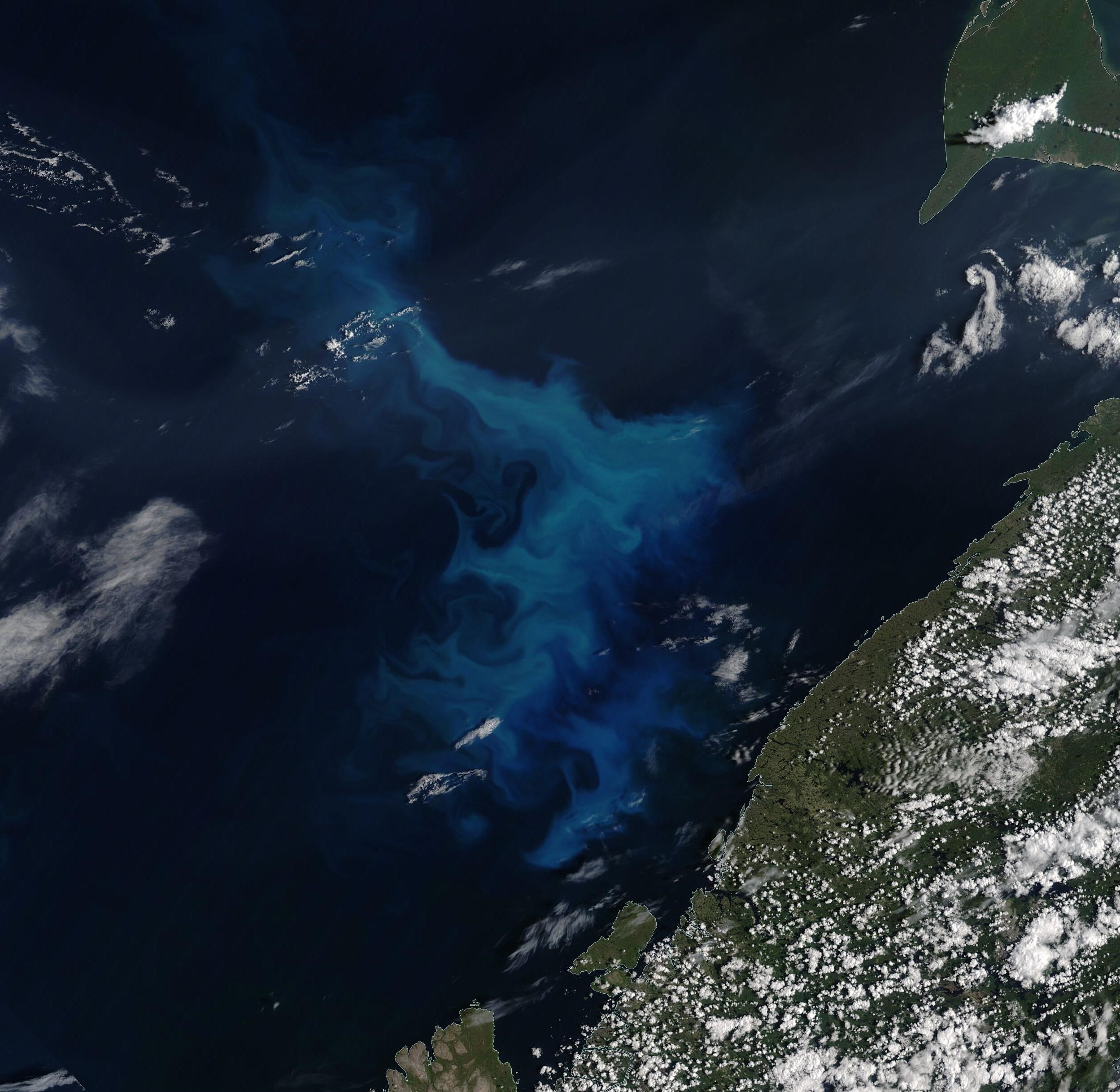
Figure 6. This image shows a phytoplankton bloom in the Barents Sea on July 26, 2020, from a Moderate Resolution Imaging Spectroradiometer (MODIS) True Color composite in NASA Worldview. The phytoplankton show up in the visible imagery as a light blue and teal swirling pattern against the dark blue ocean. The northern part of the Finnoscandian peninsula is in the lower right corner.
Credit: NASA Worldview
High-resolution image
As sea ice retreats and melt ponds form, more light can enter the Arctic Ocean, increasing the time-period over which phytoplankton can grow. This may increase overall net primary productivity, which is the rate at which the full metabolism of phytoplankton produces biomass, as light plays a strong role in initiating phytoplankton growth. Other factors may counteract the positive influence of more light availability, namely reduced mixing of deep nutrients to the surface waters. Mixing is reduced due to increased sea ice melt, precipitation and river outflow, which can increase surface stratification, or inhibit mixing, and hence inhibit nutrients from reaching the surface.
A new study analyzed 20 years of phytoplankton and net primary productivity over the Central Arctic Ocean. Researchers examined these competing effects using a combination of direct observations on light and phytoplankton biomass together with satellite-derived estimates of chlorophyll a (Chl a) and sea ice concentration. Overall, Chl a concentrations have increased for the Arctic Ocean as a whole, but there are large regional differences, with increases in Chl a observed in the Chukchi and Barents inflow shelves, and no significant changes elsewhere.
The study was able to determine that increases in net primary productivity from 1998 to 2018 were not only a result of changes in open water fraction, but also a result of changes in nutrient availability. In particular, Pacific water inflow through Bering Strait has brought more nutrients into the Chukchi Sea to support summer phytoplankton blooms. Similarly, on the Atlantic side, weakening of the mixed layer ocean stratification increased nutrient availability to surface waters. Chl a increases on shelfbreaks appears to be a result of increased vertical mixing as sea ice melts back and exposes surface waters to winds. This vertical mixing overcomes the stratification effects of the added freshwater. Overall, primary production of the Arctic Ocean has increased 57 percent between 1998 and 2018.
Antarctic check-in

Figure 7. This figure shows the Japanese Aerospace Exploration Agency (JAXA) Advanced Microwave Scanning Radiometer 2 (AMSR2) sea ice concentration for Antarctic sea ice on July 30, 2020. The Cosmonaut Sea polynya is the oblong low-concentration region near 35° East longitude.
Credit: University of Bremen
High-resolution image
Antarctic sea ice grew at a slower-than-average pace in July, resulting in a monthly mean ice extent of 15.65 million square kilometers (6.04 million square miles), or ninth lowest in the continuous satellite record. Regionally, the Bellingshausen and eastern Ross Seas, as well as a wide area south of the Indian Ocean, had below-average extents relative to the 1981 to 2010 average, and the western Weddell Sea had above-average extent. Despite the below-average extent in the Indian Ocean region, the Cosmonaut Sea once again featured a large closed polynya of about 20,000 square kilometers (7,700 square miles) at month’s end, similar to the feature we reported on in the August 2019 ASINA summary. The feature transitioned from an embayment in the ice edge to a closed polynya around July 20. The cause of the polynya is upwelling of deeper warmer water, which suppresses sea ice growth (see references below).
Further reading
Comiso, J. C. and A. L. Gordon. 1987. Recurring polynyas over the Cosmonaut Sea and the Maud Rise. Journal of Geophysical Research: Oceans. doi: 10.1029/JC092iC03p02819.
Lee, S., S. Stroeve, M. Tsamados, and A. Khan. 2020. Machine learning approaches to retrieve pan-Arctic melt ponds from visible satellite imagery. Remote Sensing of Environment. doi.10.1016/j.rse.2020.111919.
Lewis, K. M., G. L. van Dijken, and K. R. Arrigo. 2020. Changes in phytoplankton concentration now drive increased Arctic Ocean primary production. Science. doi:10.1126/science.aay8380.
Markus, T., J. C. Stroeve, and J. Miller. 2009. Recent changes in Arctic sea ice melt onset, freeze-up, and melt season length. Journal of Geophysical Research: Oceans. doi:10.1029/2009JC005436.
Prasad, T. G., J. L. McClean, E. C. Hunke, A. J. Semtner, and D. Ivanova. 2005. A numerical study of the western Cosmonaut polynya in a coupled ocean–sea ice model. Journal of Geophysical Research: Oceans. doi: 10.1029/2004JC002858.

