The pace of sea ice decline in April was near average, while sea ice extent ranked fourth lowest in the satellite record. Sea ice age mapping shows a slight increase in the amount of older ice, but the Arctic is still dominated by first-year ice, unlike during the 1990s and earlier. An intense March storm, spanning much of the Arctic Ocean, created large ice rubble piles near Utqiaġvik, Alaska, and caused difficulties for Indigenous hunters along the northwestern Alaskan coast.
Overview of conditions
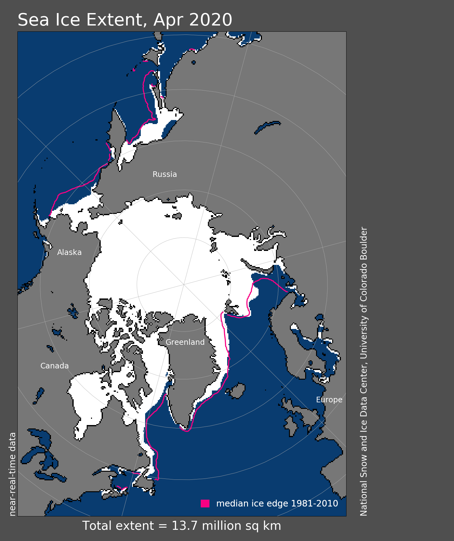
Figure 1. Arctic sea ice extent for April 2020 was 13.73 million square kilometers (5.30 million square miles). The magenta line shows the 1981 to 2010 average extent for that month. Sea Ice Index data. About the data
Credit: National Snow and Ice Data Center
High-resolution image
Arctic sea ice extent for April averaged 13.73 million square kilometers (5.30 million square miles). Last month, March ranked as the eleventh lowest ice extent in the satellite record, higher than it has been in the last five years. However, the pace of ice retreat increased toward the end of March and the ice extent in April retreated at rates similar to those seen in recent years. Consequently, ice extent for April 2020 ended up as fourth lowest—280,000 square kilometers (108,000 square miles) above the record low set in April 2019, and 960,000 square kilometers (371,000 square miles) below the 1981 to 2010 mean. As of April 30, the daily extent tracked at fourth lowest in the satellite data record.
April sea ice extent primarily retreated in the Sea of Okhotsk and the Bering Sea, but also within the Labrador Sea, Baffin Bay, the Davis Strait, and the southern end of the East Greenland Sea. However, the ice edge remained more extensive than average for this time of year in the Barents Sea between Svalbard and Novaya Zemlya, as well as in the northern East Greenland Sea. Ocean heat transport has been a good predictor of winter sea ice variability in this general region. Over the past five years, ocean temperatures have cooled in this area because of a smaller transport of warm Atlantic water from the North Atlantic. Thus, it is not surprising that the winter ice cover in this region has slowly returned from near-average to slightly above-average conditions.
Conditions in context
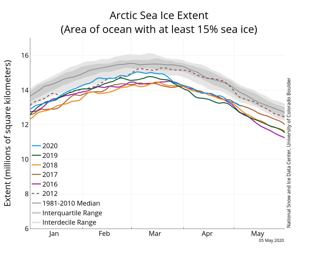
Figure 2a. The graph above shows Arctic sea ice extent as of May 5,2020, along with daily ice extent data for four previous years and the record low year. 2020 is shown in blue, 2019 in green, 2018 in orange, 2017 in brown, 2016 in purple, and 2012 in dashed red. The 1981 to 2010 median is in dark gray. The gray areas around the median line show the interquartile and interdecile ranges of the data. Sea Ice Index data.
Credit: National Snow and Ice Data Center
High-resolution image
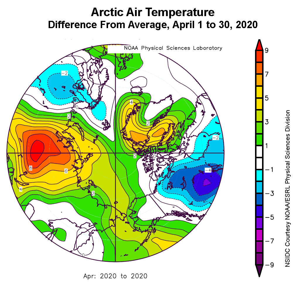
Figure 2b. This plot shows the departure from average air temperature in the Arctic at the 925 hPa level, in degrees Celsius, for April 1 to 30, 2020. Yellows and reds indicate higher than average temperatures; blues and purples indicate lower than average temperatures.
Credit: NSIDC courtesy NOAA Earth System Research Laboratory Physical Sciences Division
High-resolution image
The pace of ice loss in April was 33,400 square kilometers (12,900 square miles) per day. This was dominated by ice loss primarily in the Bering Sea and the Sea of Okhotsk, which had rates of retreat of 3,700 and 16,100 square kilometers per day (1,400 and 6,200 square miles per day), respectively. Overall, Arctic sea ice extent decreased by 1.05 million square kilometers (405,000 square miles) in April.
April air temperatures at the 925 hPa level (approximately 2,500 feet above the surface) were 2 to 5 degrees Celsius (4 to 9 degrees Fahrenheit) above average over most of the Arctic Ocean and the Bering Sea, with the exception of Svalbard and the Barents Sea where air temperatures were near average (Figure 2b). Air temperatures were also up to 6 to 8 degrees Celsius (11 to 14 degrees Fahrenheit) above average in Baffin Bay, and up to 8 degrees Celsius (14 degrees Fahrenheit) above average over Siberia, while Canada continued to experience below-average air temperatures for this time of year. This pattern of air temperatures is a result of above-average sea level pressure over Alaska and Siberia, coupled with lower pressures over the central Arctic Ocean, helping to transport warm air from the south over the Bering Sea as well as into the Kara Sea. The wind pattern also caused offshore ice motion within the Kara Sea, pushing the ice edge in the Bering Sea further north.
While 925 hPa air temperatures were above average for much of the Arctic Ocean, conditions in Utqiaġvik, Alaska, turned colder at the end of the month. On April 29, temperatures in Utqiaġvik reached -28.9 Celsius (-20 Fahrenheit), a record low for the date, according to Rick Thoman of the International Arctic Research Center in Fairbanks. It was also the latest date in the season for a temperature of -28.9 degrees Celsius (-20 degrees Fahrenheit) or lower. See below for more on unusual weather and ice events over the past couple of months in the Utqiaġvik region of Alaska.
April 2020 compared to previous years

Figure 3. Monthly April ice extent for 1979 to 2020 shows a decline of 2.65 percent per decade.
Credit: National Snow and Ice Data Center
High-resolution image
Through 2020, the linear rate of decline for April extent is 2.65 percent per decade (Figure 3). This corresponds to a trend of 38,900 square kilometers (15,000 square miles) per year.
The MOSAiC expedition continues during the pandemic

Figure 4. This figure shows the position of RV Polarstern while it is part of the Multidisciplinary drifting Observatory for the Study of Arctic Climate (MOSAiC) expedition. This position is as of April 26, 2020.
Credit: Alfred Wegener Institute
High-resolution image
Planning a year-long Arctic Ocean expedition is logistically difficult. Challenges range from finding a suitable ice floe to support the various science activities, to dealing with break up events and having to move instruments to keep them from falling into the Arctic Ocean, to extreme weather conditions. There can also be unexpected visits by polar bears and foxes. Yet, no amount of planning could have prepared the expedition for the coronavirus disease 2019 (COVID-19) pandemic. While the leg-three participants of the Multidisciplinary drifting Observatory for the Study of Arctic Climate (MOSAiC) expedition should have been home by now, the rotation of personnel via aircraft had to be cancelled. Instead, the next exchange of personnel will be at the end of May, relying on two German research vessels, RV Sonne and RV Maria S. Merian, to meet RV Polarstern at the ice edge. The Polarstern will meet the vessels near Svalbard, and after refueling and transferring the freight and people, will head back into the ice to continue the measurement program. Some equipment may be left on the ice floe while the Polarstern is away, the intent being to continue recording data.
Colleagues at the Alfred Wegener Institute (AWI) determined the origin of the ice floe selected to host most of the MOSAiC instrumentation. Satellite observations and ice drift mapping indicates that the floe formed in a polynya north of the New Siberian Islands in early December 2018. At the time the MOSAiC Central Observatory (CO) was established, the ice thickness ranged from 30 to 80 centimeters (12 to 31 inches), which is relatively thin compared to historical ice conditions. Yet recent EM-Bird sea ice thickness sensor observations from helicopter on April 10 show that the CO and the surrounding ice now have a modal thickness of around 1.8 meters (5.9 feet). Leaving valuable scientific gear on the floe is risky given the possibility that the floe will break up or be crushed while the Polarstern is away. Indeed, new leads (roughly linear openings in the ice cover) formed on April 10, and on April 27, compressive forces on the ice led to ridging. Such events raise concern that instruments may be lost or damaged while the Polarstern is away. Furthermore, during the 2019 to 2020 winter, there was a strong transpolar drift of the ice, which may require a relocation of the camp further north so that the study site does not drift out of the Arctic Ocean before the end of September. This strong ice drift appears to be related to last winter’s strongly positive phase of the Arctic Oscillation.
Impacts of a major storm on Alaska Arctic sea ice
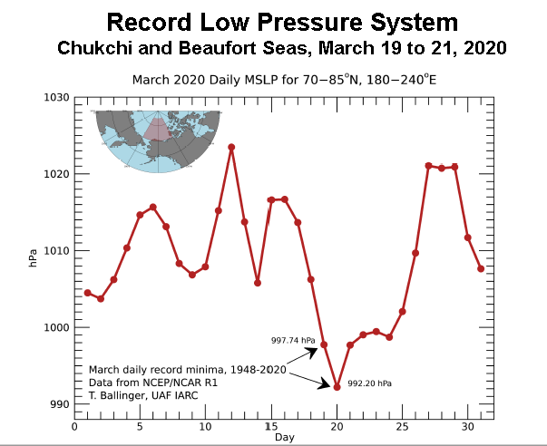
Figure 5a. This figure shows record low atmospheric mean sea-level pressure (MSLP; lowest for time period 1948 to 2020 on days indicated in graphic) north of Alaska in March 2020 during passage of major storm systems. The figure shows the daily average over the Beaufort and Chukchi Seas (shaded region in inset), which was 992.2 hPa, rather than the minimum of the center of the low, which was 970 hPa.
Credit: Tom Ballinger, International Arctic Research Center, University of Alaska Fairbanks.
High-resolution image
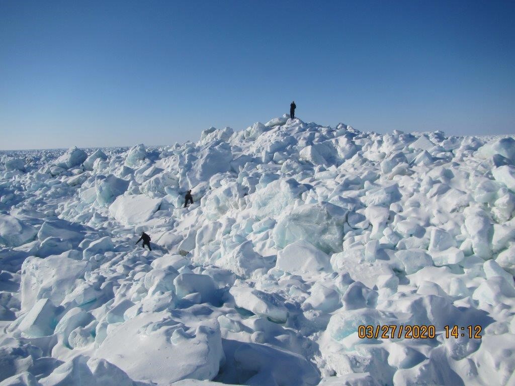
Figure 5b: This photo shows a pressure ridge formed in shorefast sea ice near Utqiaġvik, Alaska, as a result of storm-driven ice deformation.
Credit: Billy Adams of Utqiaġvik, Alaska.
High-resolution image
From March 19 to 21, a record low pressure system (Figure 5a) moved across the Chukchi and Beaufort Seas, with central pressure minimums reaching 970 hPa. Our colleague Hajo Eicken, Professor of Geophysics at the University of Alaska-Fairbanks, notes that the passage of this record low highlights the importance of major storm events in shaping the sea ice cover. A series of storms in March 2020, with peak wind speeds exceeding 97 kilometers per hour (60 miles per hour), piled up ice along the eastern Chukchi Sea coastline. Large ice pressure ridges (Figure 5b) can ground on the seafloor and help anchor the shorefast ice. They create a more stable ice platform for use by the local community to gain access to marine mammals that have been located further offshore. In recent years, milder ice conditions have resulted in less stable coastal ice. Ice deformation events due to major storms such as those that occurred this March can help make up for reduced ice growth from higher temperatures. Billy Adams, an Iñupiaq ice expert from Utqiaġvik, Alaska, reports that thicker and stronger first-year ice this winter resulted in grounding of pressure ridges further offshore than in prior recent years (Figure 5b). Community ice trails also have to extend further out from shore.
Whereas the storms piled up ice against the eastern Chukchi Sea shoreline, prevailing wind directions in the Beaufort Sea created open water and broke up large stretches of the ice pack into small floes. Break up and deformation of ice floes during passage of these storm systems threatened to disrupt a field experiment on an ice floe in the Beaufort Sea. The changing sea ice regime increasingly challenges on-ice operations and ice-based scientific research in this part of the Arctic. The absence of a strong Beaufort high pressure system in 2020 and previous years (Moore et al., 2018) has resulted in more sluggish ice movement in the Beaufort Sea. While this helps build up a thicker ice pack and makes it easier for scientific ice camps to operate in the region, it also allows for major storm systems to penetrate, wreaking havoc on the ice cover and bringing snowfall and blizzard conditions.
Update on sea ice age
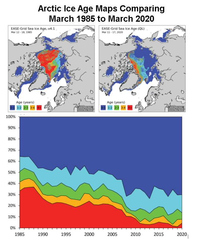
Figure 6. The top maps compare Arctic sea ice age for (a) March 12 to 18, 1985, and (b) March 11 to 17, 2020. The time series (c) of mid-March sea ice age as a percentage of Arctic Ocean coverage from 1985 to 2020 shows the nearly complete loss of 4+ year old ice; note the that age time series is for ice within the Arctic Ocean and does not include peripheral regions where only first-year (0- to 1-year-old) ice occurs, such as the Bering Sea, Baffin Bay, Hudson Bay, and the Sea of Okhotsk
Credit: W. Meier, NSIDC
High-resolution image
After the winter maximum extent, it is useful to check in on sea ice age. Older ice is generally thicker and thus less prone to melt completely during the following summer. As noted in previous years, the ice has been on average getting younger, with very little old (4+ year) ice remaining in the Arctic. During the 1980s, a substantial portion of the Arctic Ocean was covered by this old ice around the sea ice maximum (Figure 6). Last year, however, was a record low extent of 4+ year ice for this time. During the week of March 11 to 17, 326,000 square kilometers (126,000 square miles) or 4.3 percent of the ice within the Arctic Ocean was at least four years old. This is up from last year when only 91,000 square kilometers (35,000 square miles) or 1.2 percent of this old ice remained. Thus, there has been some replenishment of the oldest, thickest ice over the past year. However, the amount is still far below mid-1980 levels when over 2 million square kilometers (772,000 square miles) or around 35 percent of the Arctic Ocean was comprised of 4+-year-old ice.
The increase in the oldest ice has been offset by younger categories, one to four years old. The amount of first-year ice (0- to 1-year old) is close to the same level as last year’s, at about 70 percent of the Arctic Ocean ice cover, much higher than during the mid-1980s, when only 35 to 40 percent of the ice was less than a year old. A study of the updated ice age (and ice motion) product is being published in The Cryosphere (Tschudi et al., 2020).
Fast drifting trace elements
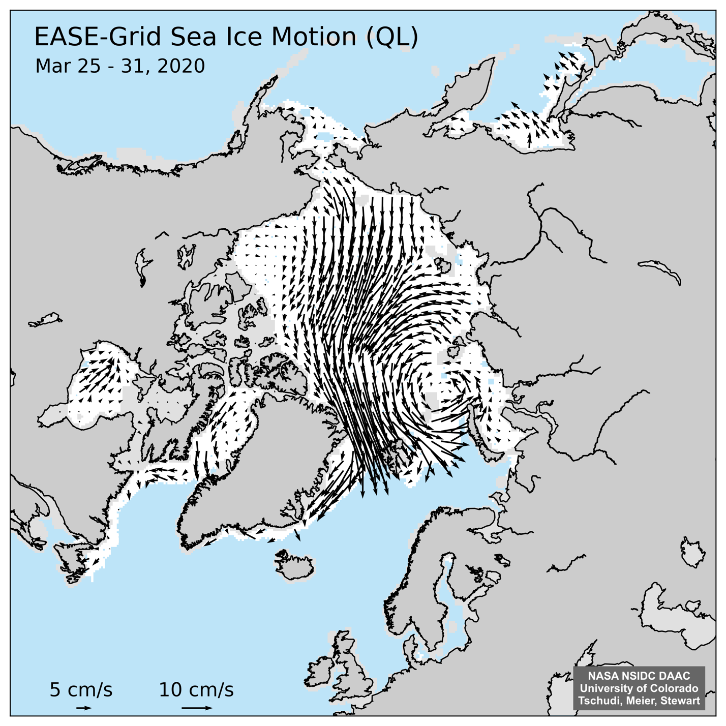
Figure 7. This figure shows ice motion from March 25 to March 31, 2020, revealing a strong Transpolar Drift and ice export towards Svalbard and out of Fram Strait.
Credit: National Snow and Ice Data Center
High-resolution image
The Transpolar Drift Stream, a general motion of ice from shores of Siberia, across the Pole and then towards Fram Strait, was enhanced during the extreme positive phase of the Arctic Oscillation this winter. A new study found that freshwater runoff from rivers around the western Arctic Ocean (Siberia, Alaska, and northwestern Canada) brings significant amounts of trace elements into the Arctic Ocean through the Transpolar Drift Stream. Trace elements entering the Arctic Ocean from rivers are chemically bound with organic matter in the rivers, which allows them to be transported long distances. The Transport Drift Stream can then take those trace elements across the Arctic Ocean and towards Fram Strait. This may have important implications for marine ecosystems. One key element, iron, is a key nutrient for primary productivity (e.g., algae growth). More iron transported into the Arctic Ocean and more sunlight from reduced sea ice extent can enhance productivity. As permafrost thaws and more nutrients are released, this could become an important component of change in marine ecosystems in the future.
Antarctica sea ice near average
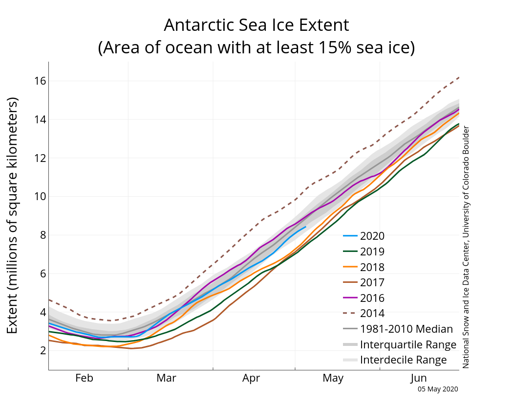
Figure 8a. The graph above shows Antarctic sea ice extent as of May 5, 2020, along with daily ice extent data for four previous years and the record high year. 2020 is shown in blue, 2019 in green, 2018 in orange, 2017 in brown, 2016 in purple, and 2014 in dashed brown. The 1981 to 2010 median is in dark gray. The gray areas around the median line show the interquartile and interdecile ranges of the data. Sea Ice Index data.
Credit: National Snow and Ice Data Center
High-resolution image

Figure 8b. This figure shows Antarctic regional extent over the last 12 months. Antarctic regional extent over the last 12 months—May 1, 2019, through April 30, 2020. Regions are noted in the map inset (“Bell.-Amund. Seas” refers to the Bellingshausen and Amundsen Seas).
Credit: National Snow and Ice Data Center
High-resolution image
Antarctic sea ice extent tracked close to the median line from mid-March until the first week of April when the rate of growth fell below the median rate and the trend returned to the lower end of the observed 41-year range. However, it remained within the interdecile range. Sea ice extent is near average in most sectors, but is slightly below average in the Ross Sea, parts of the Weddell Sea, and off the coast of Dronning Maud Land.
NSIDC has recently published regional ice extent and concentration spreadsheets for five sectors of the Southern Ocean surrounding Antarctica. These allow users to quickly examine how sea ice is varying in different regions. This is similar to the regional spreadsheets previously available for the Arctic.
The regional spreadsheets are illustrative of how the seasonal cycle varies in different parts of the Antarctic. For example, as shown for the past year, the seasonal variation is dominated by the changes in the Weddell Sea, going from a maximum of around 7 million square kilometers (2.70 million square miles) in late August to just over 1 million square kilometers (386,000 square miles), with a very sharp decline during December 2019. Significant seasonal ice retreat starts first in the Indian Ocean region in late September, with a very short transition between advance and retreat. Other regions show less seasonal variability. Notably, the dates of the maximums of the regions varies over a couple months, but all reach a minimum at nearly the same time—end of February to early March.
Future reading
Årthun, M., T. Eldevik, and L. H. Smedsrud. 2019. The Role of Atlantic Heat Transport in Future Arctic Winter Sea Ice Loss. Journal of Climate. doi:10.1175/JCLI-D-18-0750.1.
Charette, M. A., L. E. Kipp, L. T. Jensen, J. S. Dabrowski, L. M. Whitmore, J. N. Fitzsimmons, et al. 2020. The Transpolar Drift as a Source of Riverine and Shelf‐Derived Trace Elements to the Central Arctic Ocean. Journal of Geophysical Research: Oceans. doi:10.1029/2019JC015920
Krumpen, T., et al. 2020. The MOSAiC ice floe: sediment-laden survivor from the Siberian shelf. The Cryosphere. doi:10.5194/tc-2020-64.
Moore, G. W. K., A. Schweiger, J. Zhang, and M. Steele. 2018. Collapse of the 2017 winter Beaufort High: A response to thinning sea ice? Geophysical Research Letters. doi:10.1002/2017GL076446
Tschudi, M. A., W. N. Meier, and J. S. Stewart. 2020. An enhancement to sea ice motion and age products at the National Snow and Ice Data Center. The Cryosphere. doi.10.5194/tc-14-1519-2020.

