After reaching its annual maximum on March 5, Arctic sea ice extent remained stable for several days before it started clearly declining. Continuing the pattern of this past winter, the Arctic Oscillation was in a persistently positive phase. Scientists participating in the Multidisciplinary drifting Observatory for the Study of Arctic Climate (MOSAiC) expedition finally reached shore after being held at sea for three weeks from a combination of logistical challenges and COVID-19 concerns.
Overview of conditions

Figure 1. Arctic sea ice extent for March 2020 was 14.78 million square kilometers (5.71 million square miles). The magenta line shows the 1981 to 2010 average extent for that month. Sea Ice Index data. About the data
Credit: National Snow and Ice Data Center
High-resolution image
The March 2020 Arctic sea ice extent was 14.78 million square kilometers (5.71 million square miles). This was the eleventh lowest in the satellite record, 650,000 square kilometers (251,000 square miles) below the 1981 to 2020 March average and 490,000 square kilometers (189,000 square miles) above the record low March extent in 2017.
At the end of the month, extent was particularly low in the Bering Sea after a rapid retreat during the second half of the month. Ice loss was also prominent in the Sea of Okhotsk and Gulf of St. Lawrence.
Conditions in context
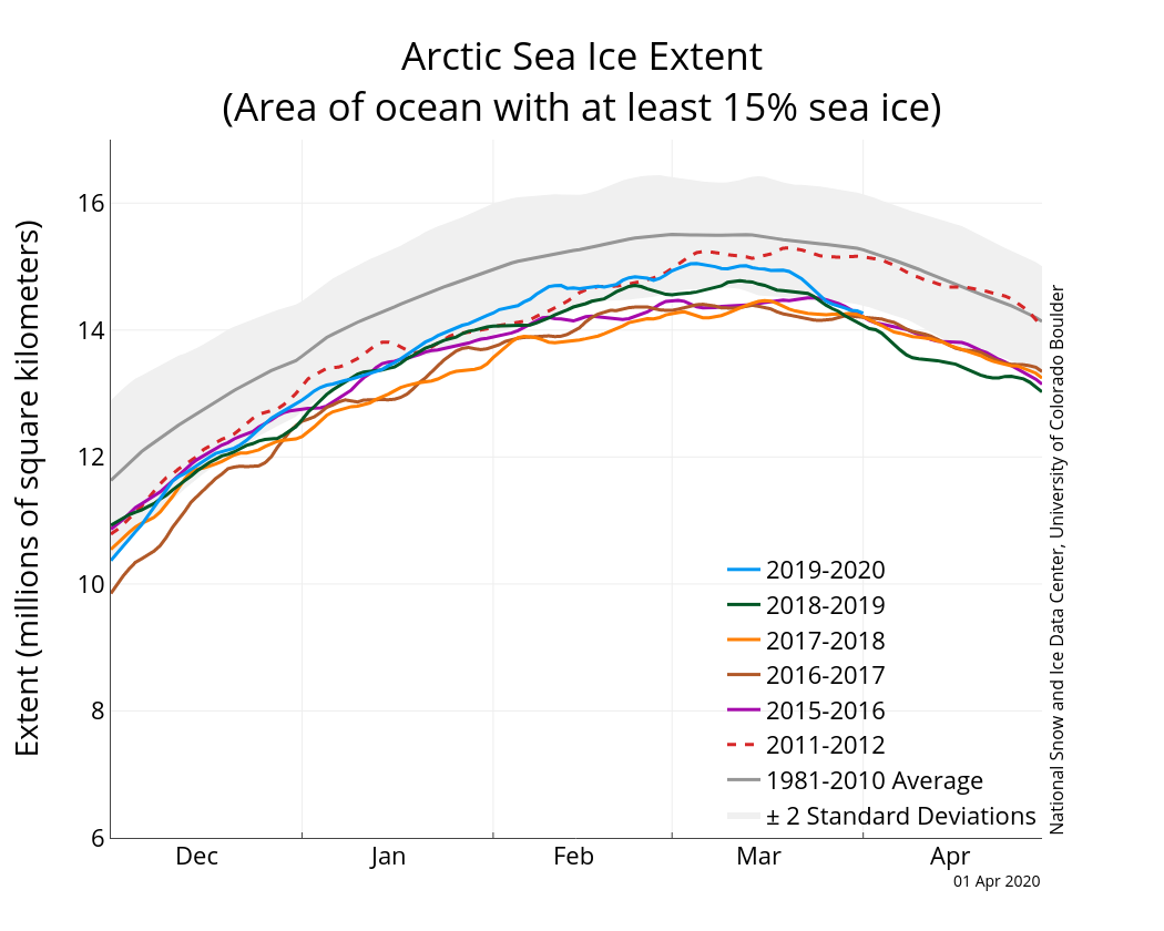
Figure 2a. The graph above shows Arctic sea ice extent as of April 1, 2020, along with daily ice extent data for four previous years and the record low year. 2019 to 2020 is shown in blue, 2018 to 2017 in green, 2017 to 2016 in orange, 2016 to 2017 in brown, 2015 to 2016 in purple, and 2011 to 2012 in dashed red. The 1981 to 2010 median is in dark gray. The gray areas around the median line show the interquartile and interdecile ranges of the data. Sea Ice Index data.
Credit: National Snow and Ice Data Center
High-resolution image
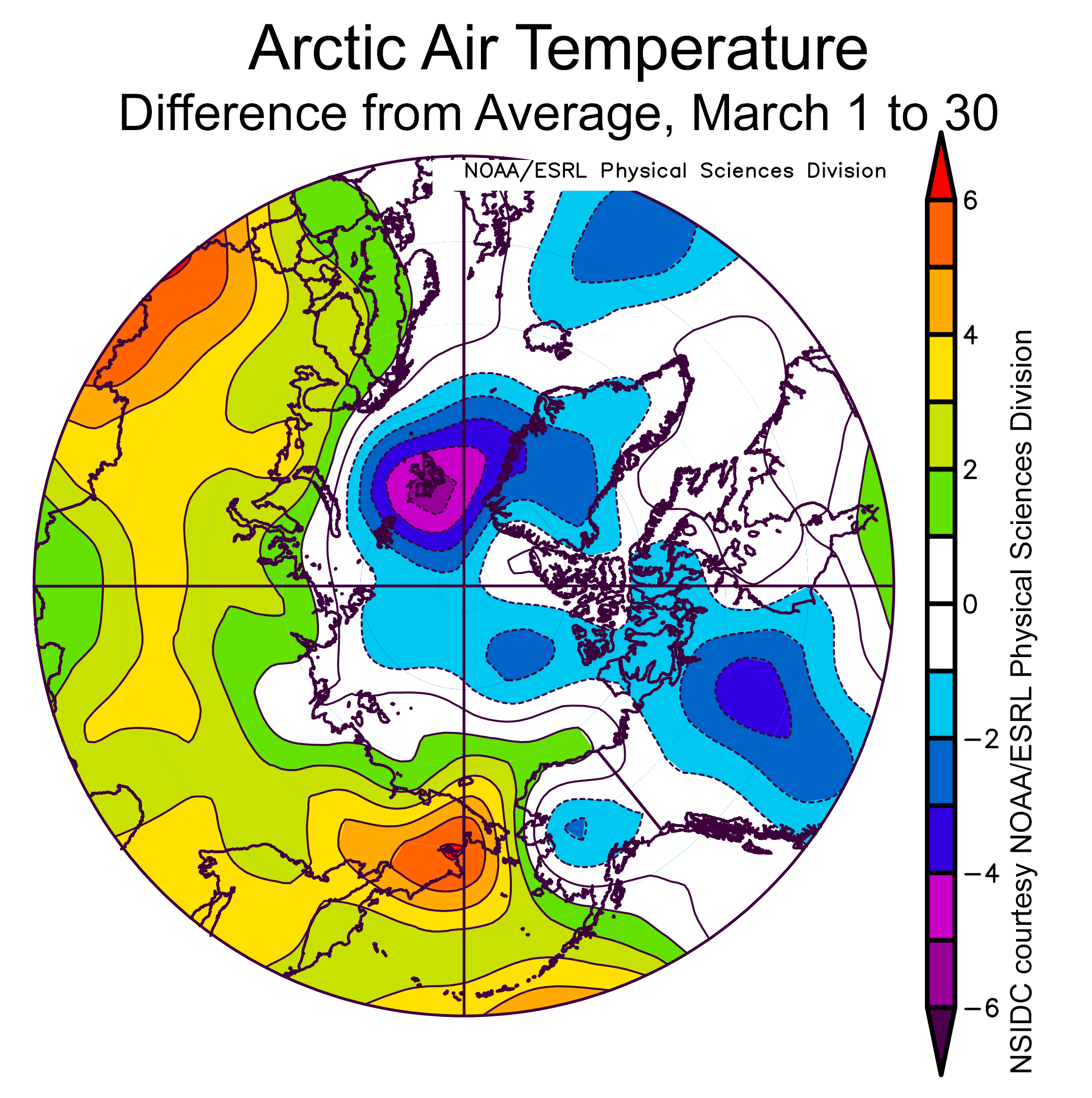
Figure 2b. This plot shows the departure from average air temperature in the Arctic at the 925 hPa level, in degrees Celsius, for March 1 to 30, 2020. Yellows and reds indicate higher than average temperatures; blues and purples indicate lower than average temperatures.
Credit: NSIDC courtesy NOAA Earth System Research Laboratory Physical Sciences Division
High-resolution image
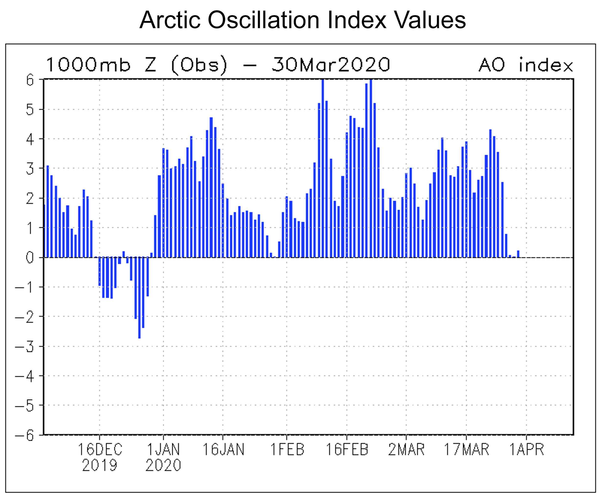
Figure 2c. The plot shows the values of the Arctic Oscillation Index, which is a weather phenomenon indicating the state of the atmospheric circulation over the Arctic.
Credit: National Centers for Environmental Prediction/National Oceanic and Atmospheric Administration
High-resolution image
After reaching its maximum on March 5, extent declined slowly until March 19 after which it declined rapidly for the next ten days. The decrease was most pronounced in the Bering Sea, where extent went from slightly above average at the time of the maximum to well below average by the end of the month. Overall, sea ice extent decreased 750,000 square kilometers (290,000 square miles) between March 5 and March 31, with 590,000 square kilometers (228,000 square miles) of this decrease occurring between March 19 and March 29.
Air temperatures in March at the 925 hPa level (approximately 2,500 feet above the surface) over the Arctic Ocean were near average to slightly below average (Figure 2b). Temperatures over the central Arctic Ocean were 2 to 3 degrees Celsius (4 to 5 degrees Fahrenheit) below average, but as much as 6 degrees Celsius (11 degrees Fahrenheit) below average in the region around Svalbard. Only in the Sea of Okhotsk and the Bering Sea were temperatures above average (2 to 5 degrees Celsius or 4 to 9 degrees Fahrenheit). Sea level pressure was very low over the Arctic Ocean, reflecting the strong positive mode of the Arctic Oscillation (AO) that has persisted through most of the past winter (Figure 2c). The AO index became more neutral by the end of March but has been positive through all of 2020 so far.
March 2020 compared to previous years
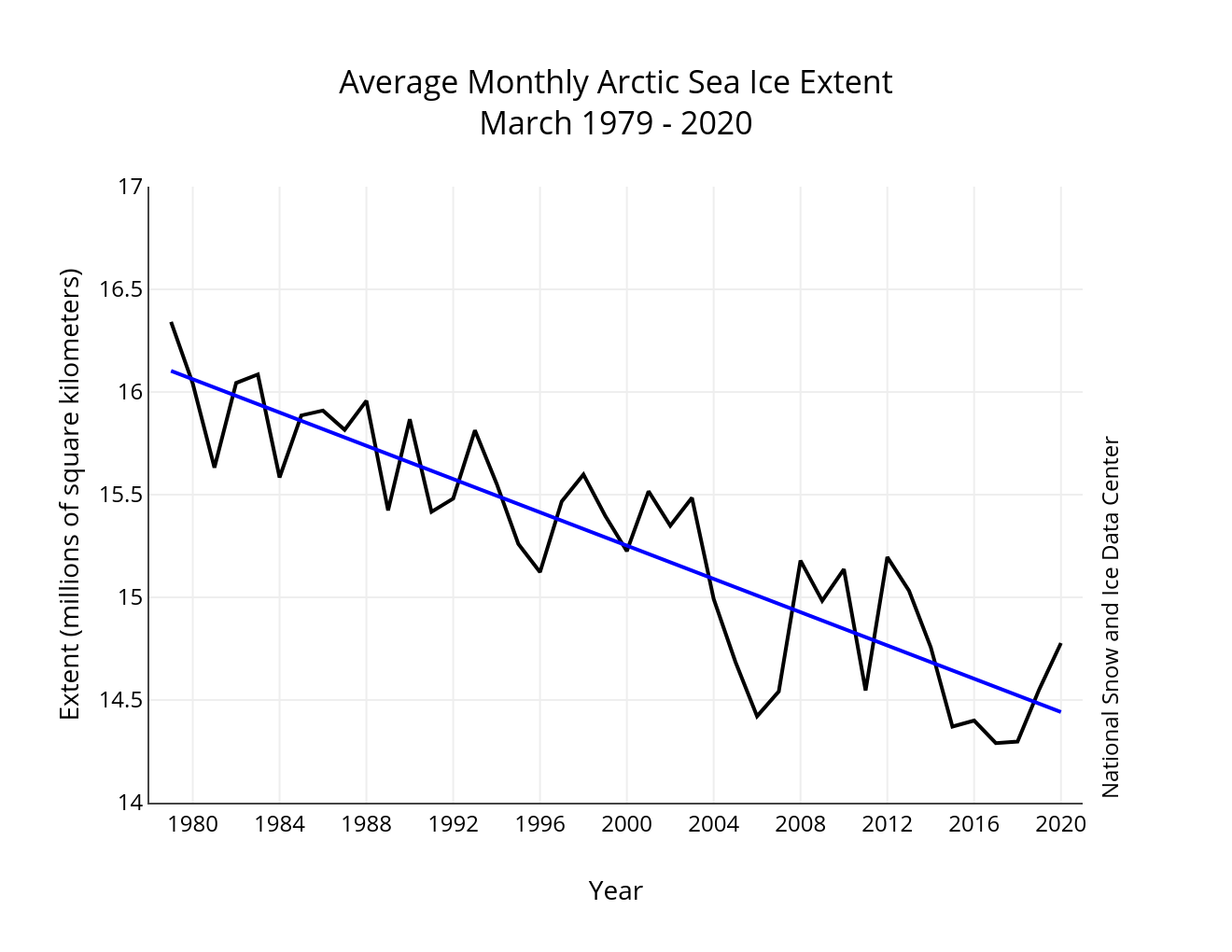
Figure 3. Monthly March ice extent for 1979 to 2020 shows a decline of 2.6 percent per decade.
Credit: National Snow and Ice Data Center
High-resolution image
Through 2020, the linear rate of decline for March extent is 2.6 percent per decade. This corresponds to a trend of 40,500 square kilometers (15,600 square miles) per year, which is roughly the size of Massachusetts and Connecticut combined. Over the 42-year satellite record, the Arctic has lost about 1.66 million square kilometers (641,000 square miles) of sea ice in March, based on the difference in linear trend values in 2020 and 1979. This is comparable in size to the size of the state of Alaska.
Thickness data from CryoSat-2
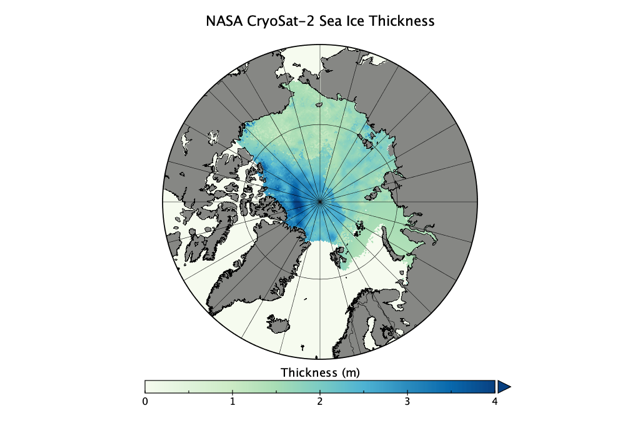
Figure 4a. This maps shows sea ice thickness for February 22, 2020. Light green depicts ice under a meter thin; dark blue depicts ice up to 4 meters thick. NASA Goddard (Kurtz and Harbeck, 2017) produces the thickness product and the NASA NSIDC Distributed Active Archive Center distributes it.
Credit: W. Meier, NSIDC
High-resolution image
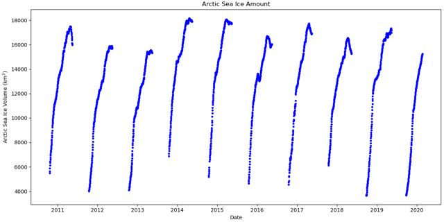
Figure 4b. This graph shows sea ice volume from European Space Agency (ESA) CryoSat-2 satellite from October 20, 2010 through February 22, 2020. Ice volume is tracked between mid-October and mid-May. Ice volume is estimated from the NASA CryoSat-2 Sea Ice Elevation, Freeboard, and Thickness, Version 1 product (Kurtz and Harbeck, 2017).
Credit: B. Raup, NSIDC
High-resolution image
NASA Goddard produces sea ice thickness estimates based on data from the European Space Agency CryoSat-2 radar altimeter. The altimeter sends out radar pulses that reflect from the surface back to the satellite. By measuring the time it takes for the pulses to transmit to the surface and reflect back to the satellite, the elevation of the surface can be estimated. For sea ice, this corresponds to the freeboard—the part of the ice above the waterline. Using information about snow depth, and snow and sea ice density, total thickness can be estimated.
Maps of ice thickness are produced daily with about a 40-day lag, necessary to carefully process the data (Figure 4a). CryoSat-2 has been operating since 2010, providing nearly a decade long record of sea ice thickness and sea ice volume. Ice volume roughly triples from mid-October to mid-May due to the increase in extent and thickness through the winter (Figure 4b). However, the radar altimeter cannot obtain reliable estimates over sea during summer as surface melt contaminates the radar signal.
The future of pollutant transport via sea ice drift
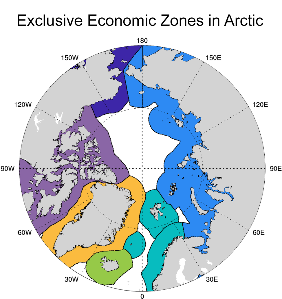
Figure 5. This map show the exclusive economic zones (EEZs) within the Arctic: Canada (purple), Greenland (orange), Iceland (green), Norway (turquoise), Russia (light blue), and USA (dark blue). As sea ice reduces there will be more opportunity for ice to drift from one EEZ to another, which has implications for the potential spread of pollutants.
Credit: DeRepentigny et al., 2020
High-resolution image
As the Arctic sea ice cover becomes less extensive, thinner, and more mobile, ice floes are able to travel longer distances in a shorter amount of time. Patricia DeRepentigny, a PhD candidate at the University of Colorado, led a study that uses the National Center for Atmospheric Research (NCAR) Community Earth System Model (CESM) to assess how the transport of sea ice across the Arctic Ocean will likely change throughout the twenty-first century. She performed CESM experiments with two different greenhouse gas emissions scenarios to assess the impact of societal choices. The area of sea ice exchanged between the different countries bordering the Arctic more than triples between the end of the twentieth century and the middle of the twenty-first century, with the Central Arctic Ocean joining the Russian coast as a major ice exporter. At the same time, the sea ice that drifts over long distances is predicted to diminish in favor of shorter drifts between neighboring Arctic countries. By the end of the twenty-first century, there are large differences between the two CESM experiments: in the high-emissions scenario, the proportion of sea ice leaving each region starts to reduce, whereas it continues to increase in the low-emissions scenario. This is because the Arctic Ocean goes completely ice free every summer under the high-emissions scenario, allowing ice floes less than a year to travel. The study raises concerns regarding risks associated with contaminants transported on distributed ice floes, especially in light of increased shipping and offshore development in the Arctic.
The return: MOSAiC update
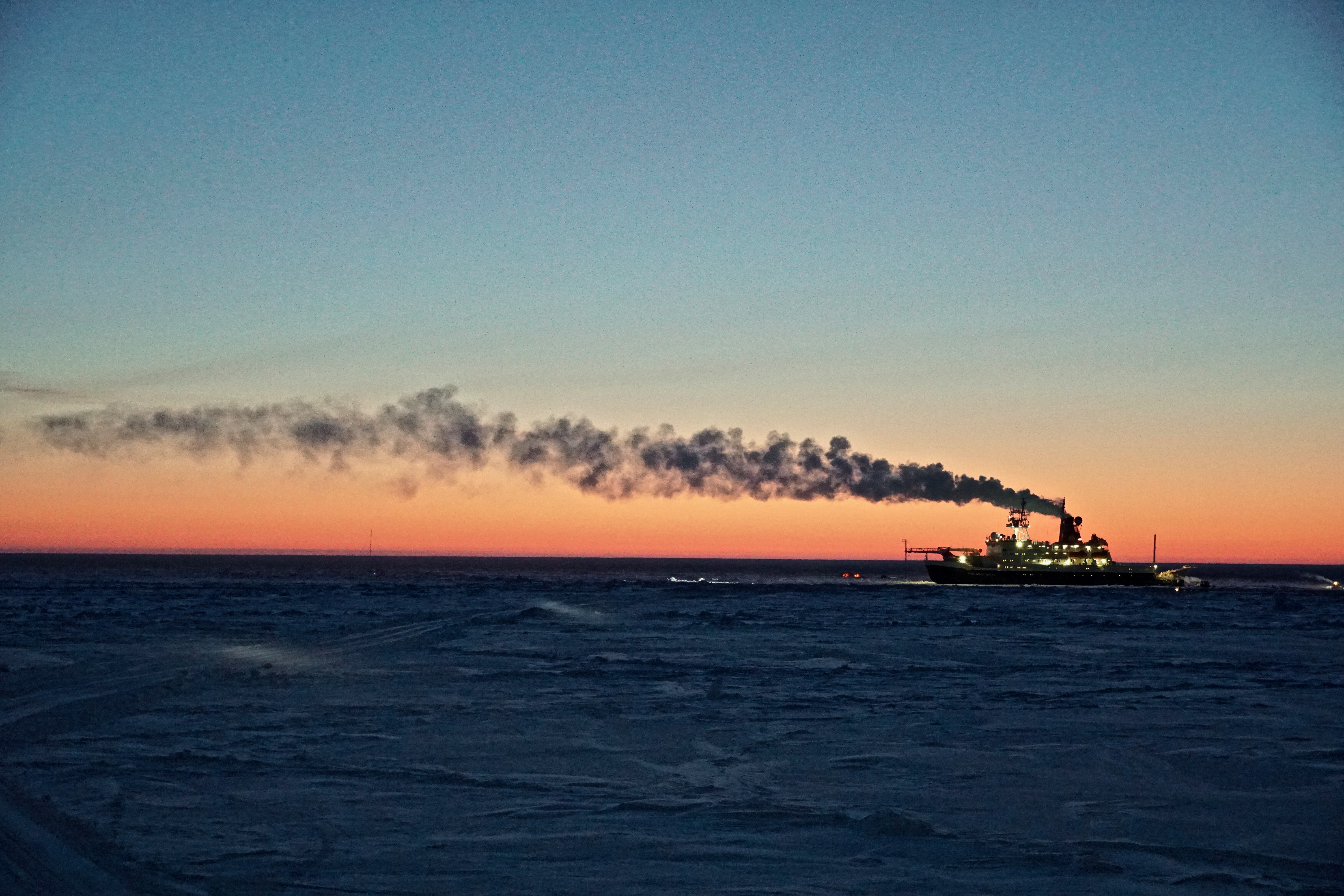
Figure 6a. The German icebreaker Polarstern drifts with the sea ice, where it has been lodged since September 2019 as part of the Multidisciplinary drifting Observatory for the Study of Arctic Climate (MOSAiC) project. As the project heads into spring, a perpetual sunrise eclipses the horizon.
Credit: J. Stroeve, NSIDC
High-resolution image
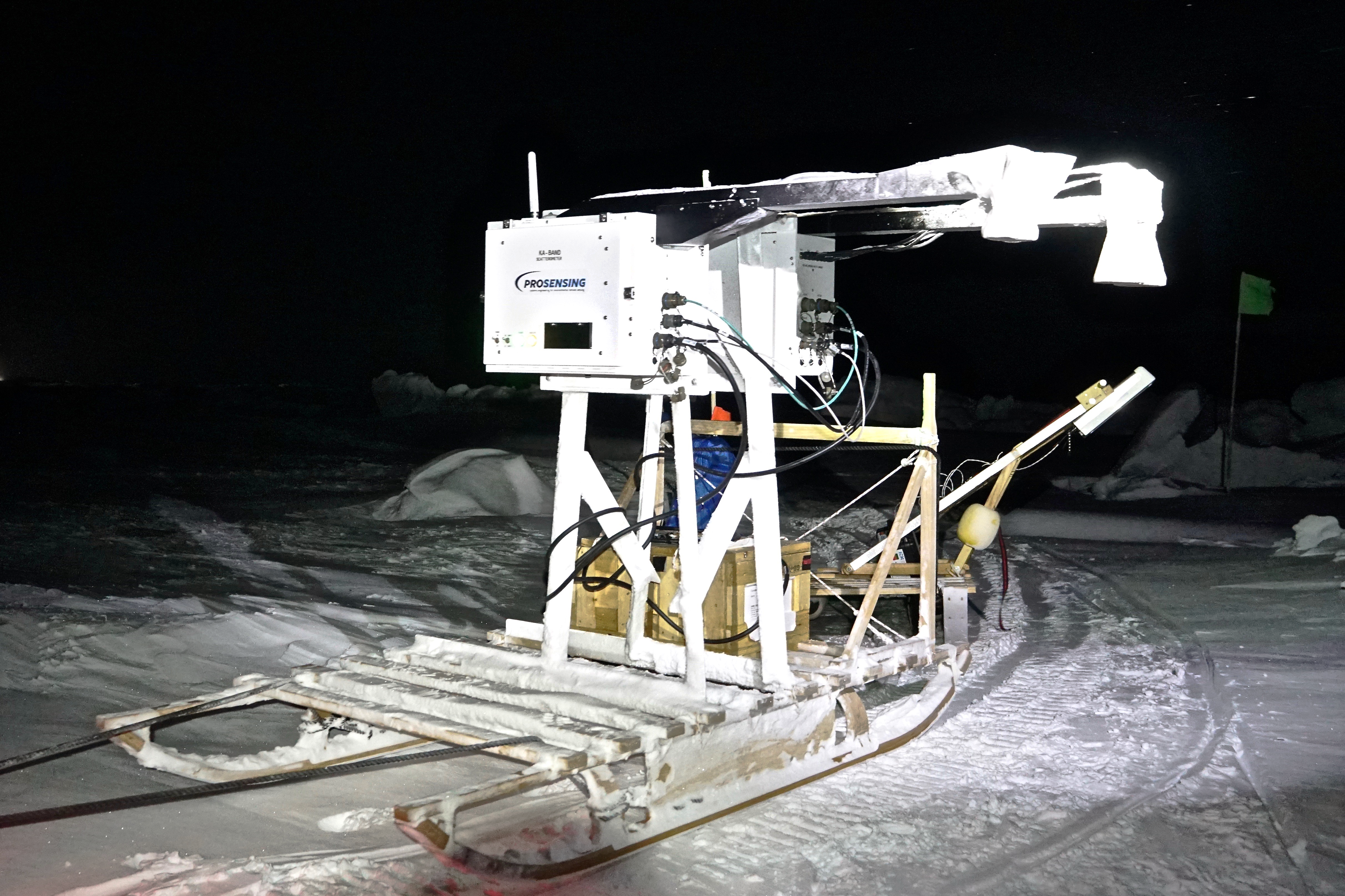
Figure 6b. The Ka/Ku radar is strapped to a tow-sled, looking straight down to simulate what a satellite altimeter would see when towed along the transects. This instrument was built by ProSensing specifically for the Multidisciplinary drifting Observatory for the Study of Arctic Climate (MOSAiC) expedition.
Credit: J. Stroeve, NSIDC
High-resolution image
After delays related to logistical challenges and the COVID-19 pandemic, the science crew of the second leg of the Multidisciplinary drifting Observatory for the Study of Arctic Climate (MOSAiC), including NSIDC scientist Julienne Stroeve, is finally back on shore. Stroeve and colleagues embarked on a supporting icebreaker on November 27, reaching the German Polarstern icebreaker—the basecamp for MOSAiC—on December 13. On leg two, Stroeve’s research focused on remote sensing of sea ice using various instruments, including a dual frequency Ka/Ku band polarimetric radar. This instrument was deployed at the remote sensing site, which consisted of a refrozen melt pond, and hourly measurements were collected. At the beginning of the instrument set up in October, the ice floe was about 80 centimeters (2.6 feet) thick but grew to nearly 2 meters (6.6 feet) thick by the end of February. The instrument was also towed along several kilometer-long transects using a sled that fixed the instrument position in a nadir (“stare”) mode to simulate returns seen by a radar altimeter (Figure 6b). The radar backscatter data will be useful to better understand how snowpack properties influence radar penetration and if a satellite radar altimeter mission using Ka- and Ku-bands can allow scientists to simultaneously map snow depth and ice thickness.
An update from the south
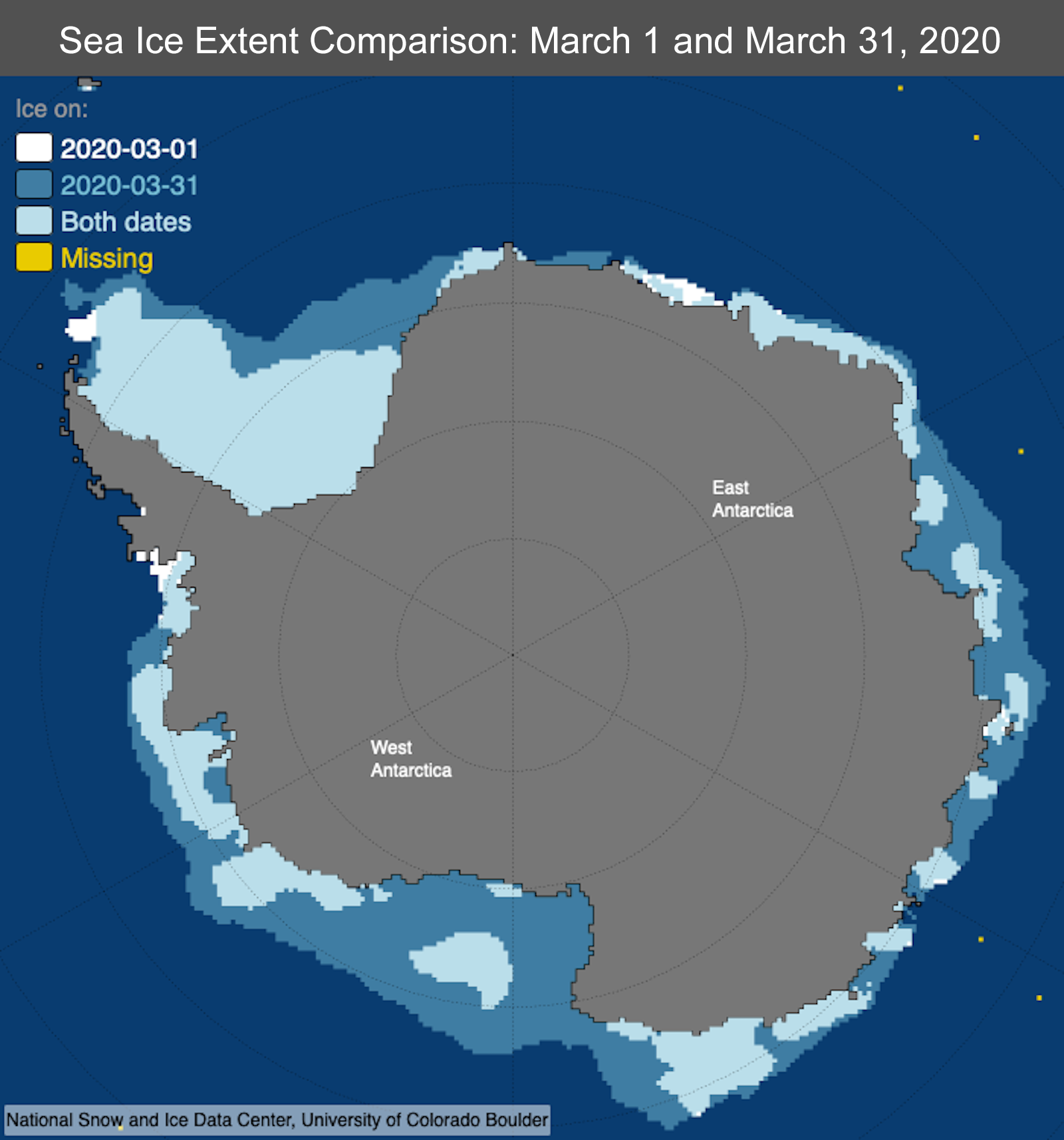
Figure 7. This map compares sea ice extent in Antarctica on March 1 and March 31, 2020.
Credit: National Snow and Ice Data Center
High-resolution image
In the Antarctic, sea ice extent has increased sharply since early March and at the end of the month is near the 1981 to 2010 average. This ends a 41-month period of below-average monthly sea ice extent. Ice growth has occurred all along the Antarctic coast, but most notably in the Ross Sea and eastern Weddell Sea regions. Air temperatures over most coastal areas for the month were near average within 1 degree Celsius (2 degrees Fahrenheit) of the 1981 to 2010 average, slightly above average near the southern Peninsula area at 1 to 3 degrees Celsius (2 to 5 degrees Fahrenheit), and notably below average in the Wilkes Land area of the ice sheet at 5 to 7 degrees Celsius (9 to 13 degrees Fahrenheit). The atmospheric circulation patterns were somewhat unusual, dominated by extensive low pressure in the Amundsen Sea and Ross Sea region, and another area of low pressure north of Dronning Maud Land. Offshore winds guided by these low-pressure areas correlate with the two areas of more rapid ice growth. Consistent with the strong low pressure in the Ross and Amundsen Seas, the Southern Annular Mode index was positive for the month.
References
DeRepentigny, P., A. Jahn, L. B. Tremblay, R. Newton, and S. Pfirman. 2020. Increased transnational sea ice transport between neighboring Arctic states in the 21st century. Earth’s Future, 8, e2019EF001284, doi.org:10.1029/2019EF001284.
Kurtz, N. and J. Harbeck. 2017. CryoSat-2 Level-4 Sea Ice Elevation, Freeboard, and Thickness, Version 1. Boulder, Colorado USA. NASA National Snow and Ice Data Center Distributed Active Archive Center. doi:10.5067/96JO0KIFDAS8.

