Daily Arctic sea ice extents for May 2016 tracked two to four weeks ahead of levels seen in 2012, which had the lowest September extent in the satellite record. Current sea ice extent numbers are tentative due to the preliminary nature of the DMSP F-18 satellite data, but are supported by other data sources. An unusually early retreat of sea ice in the Beaufort Sea and pulses of warm air entering the Arctic from eastern Siberia and northernmost Europe are in part driving below-average ice conditions. Snow cover in the Northern Hemisphere was the lowest in fifty years for April and the fourth lowest for May. Antarctic sea ice extent grew slowly during the austral autumn and was below average for most of May.

Overview of conditions

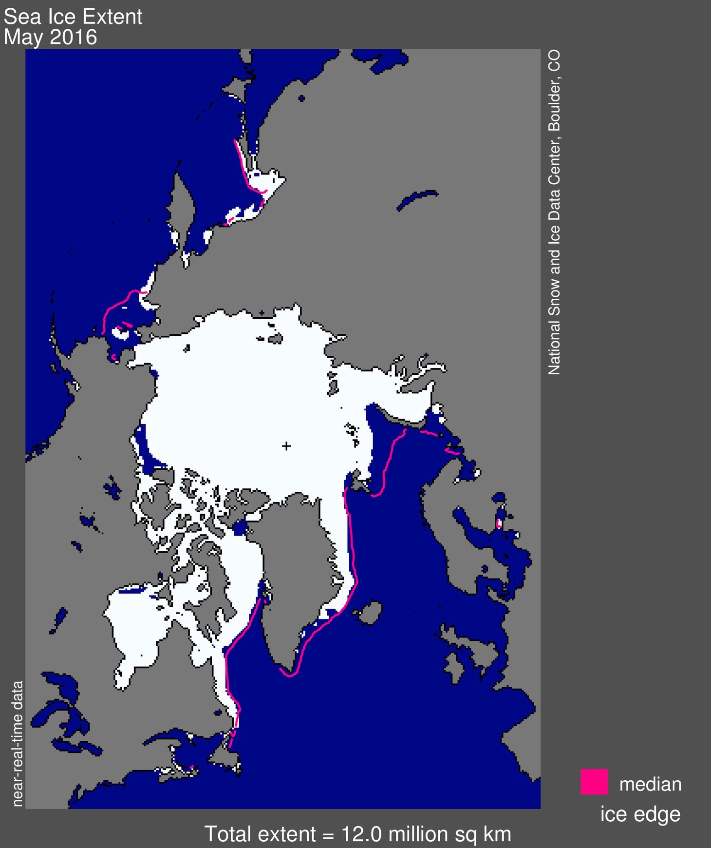
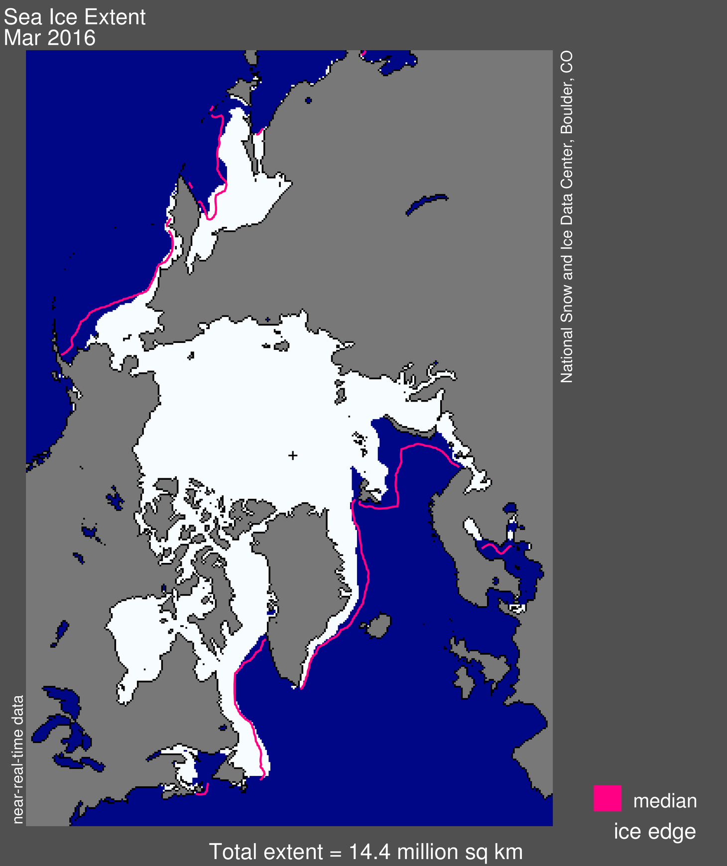
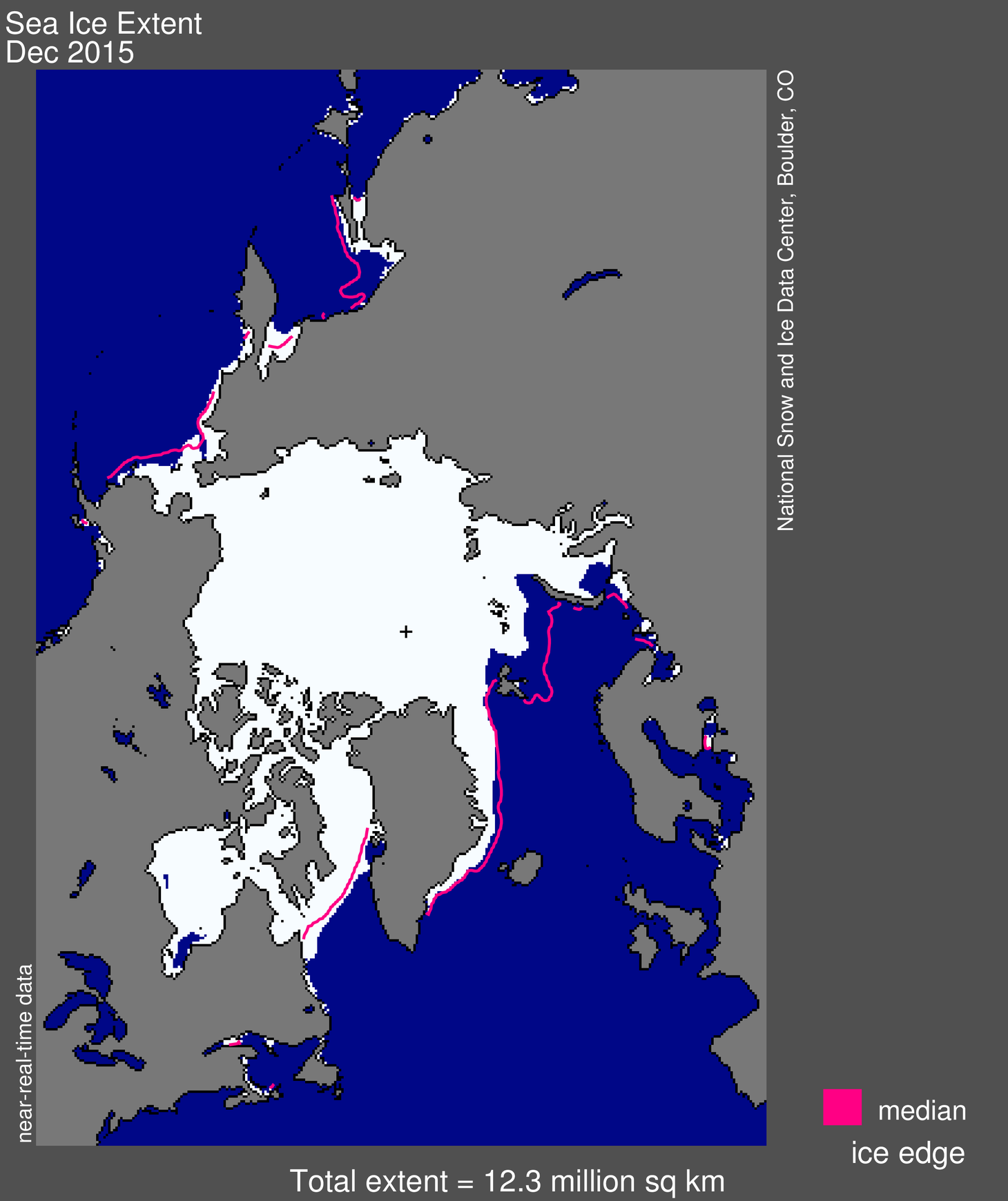
Figure 1. Arctic sea ice extent for May 2016 was 12.0 million square kilometers (4.63 million square miles). The magenta line shows the 1981 to 2010 median extent for that month. The black cross indicates the geographic North Pole. Provisional data. Not a Sea Ice Index product.

Credit: National Snow and Ice Data Center
High-resolution image

May 2016 set a new record low for the month for the period of satellite observations, at 12.0 million square kilometers (4.63 million square miles), following on previous record lows this year in January, February, and April. May’s average ice extent is 580,000 square kilometers (224,000 square miles) below the previous record low for the month set in 2004, and 1.39 million square kilometers (537,000 square miles) below the 1981 to 2010 long-term average.

During the month, daily sea ice extents tracked about 600,000 square kilometers (232,000 square miles) below any previous year in the 38-year satellite record. Daily extents in May were also two to four weeks ahead of levels seen in 2012, which had the lowest September extent in the satellite record. The monthly average extent for May 2016 is more than one million square kilometers (386,000 square miles) below that observed in May 2012.

Sea ice extent remains below average in the Kara and Barents seas, continuing the pattern seen throughout winter 2015 and 2016. Sea ice also remains below average in the Bering Sea and the East Greenland Sea. In the Beaufort Sea, large open water areas have formed near the coast and ice to the north is strongly fragmented due to wind-driven divergence. The opening began in February, continued through March, and greatly expanded in April.

Conditions in context

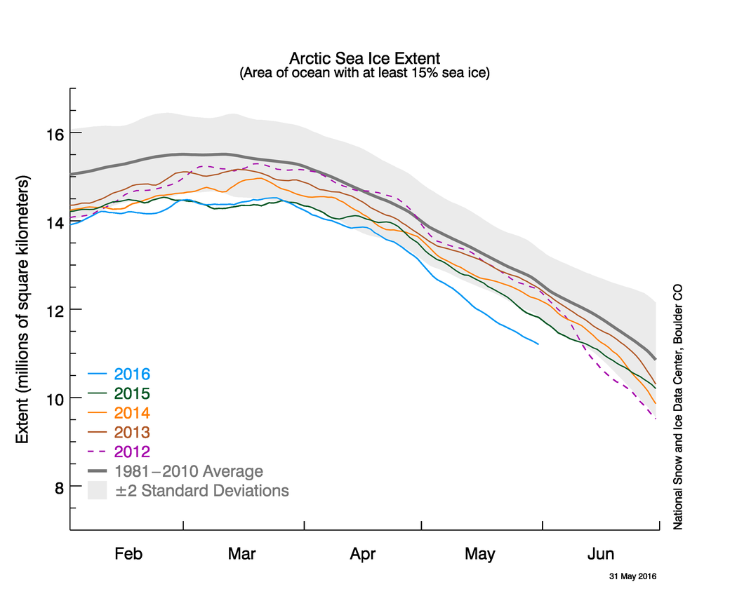
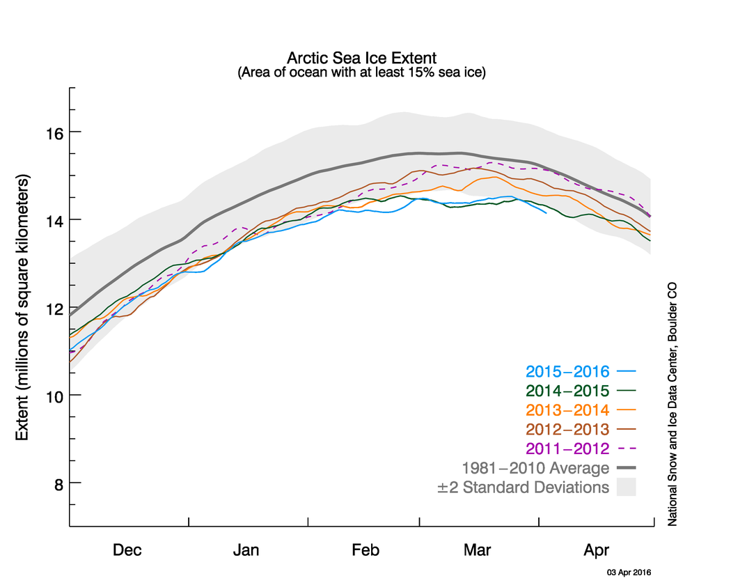
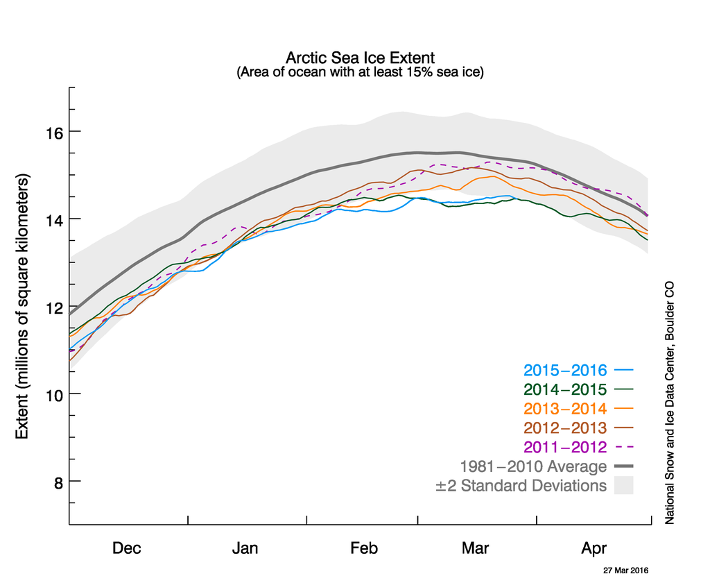
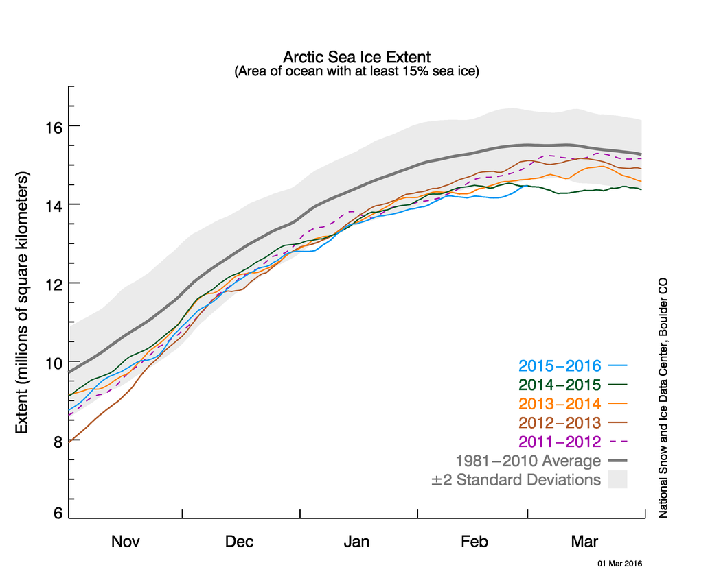
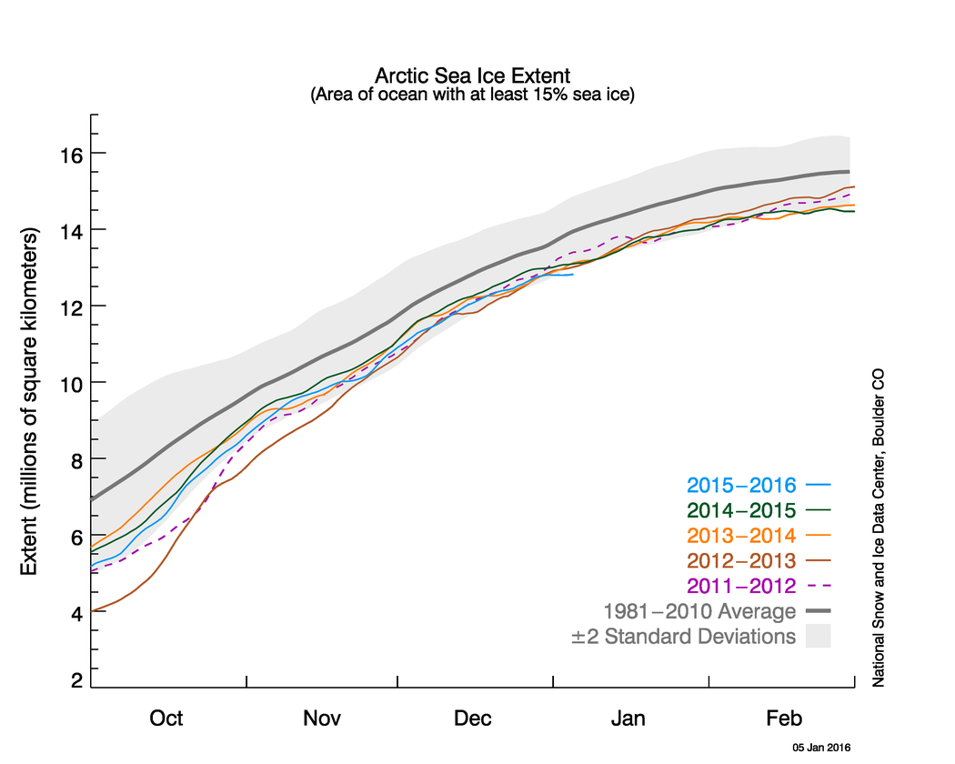
Figure 2. The graph above shows Arctic sea ice extent as of May 31, 2016, along with daily ice extent data for four previous years. 2016 is shown in blue, 2015 in green, 2014 in orange, 2013 in brown, and 2012 in purple. The 1981 to 2010 average is in dark gray. The gray area around the average line shows the two standard deviation range of the data. Provisional data. Not a Sea Ice Index product.

Credit: National Snow and Ice Data Center
High-resolution image

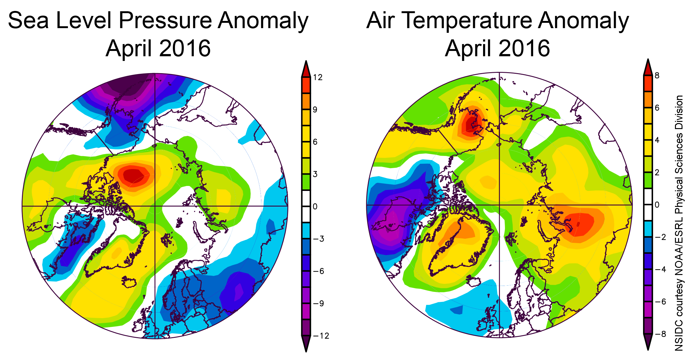
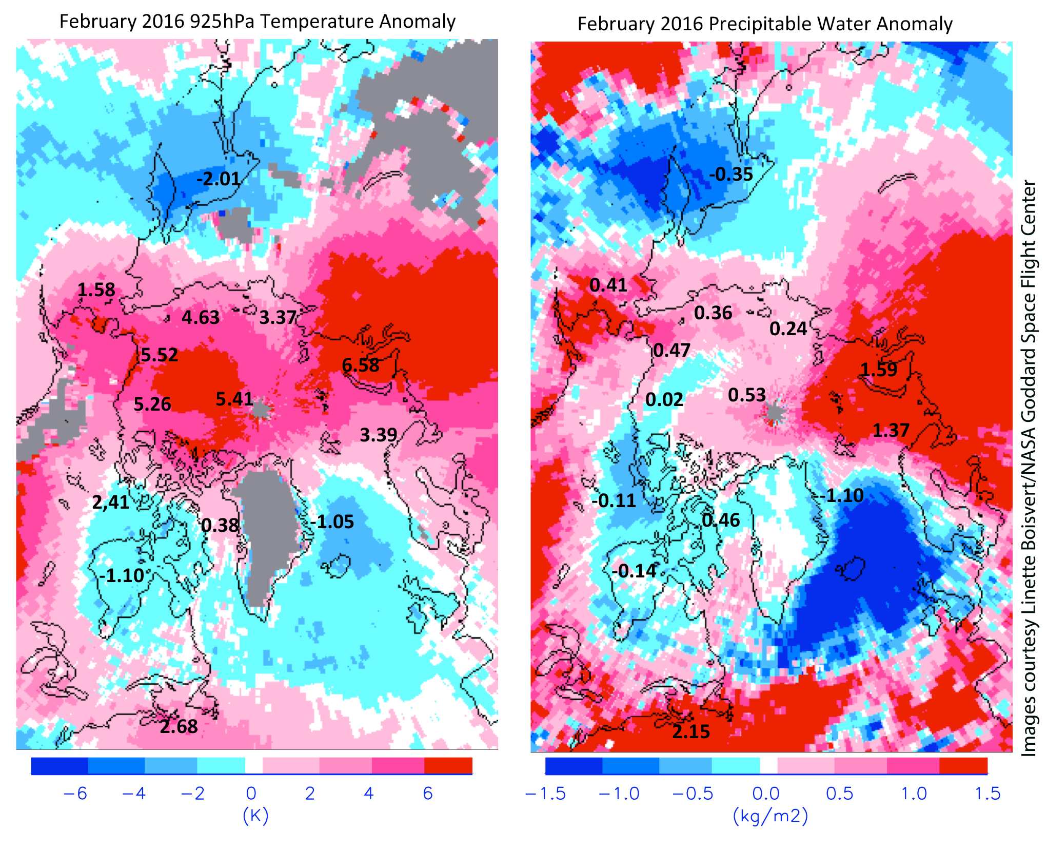
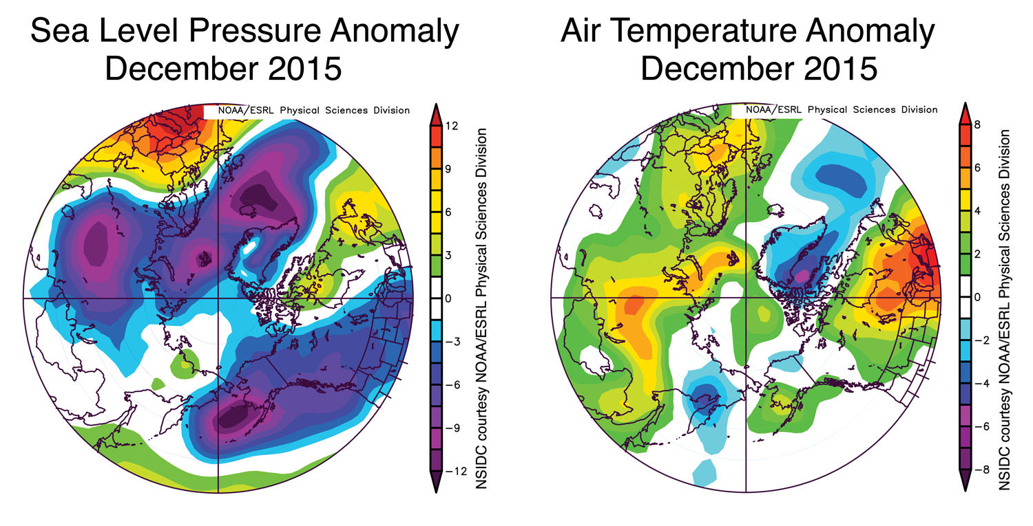
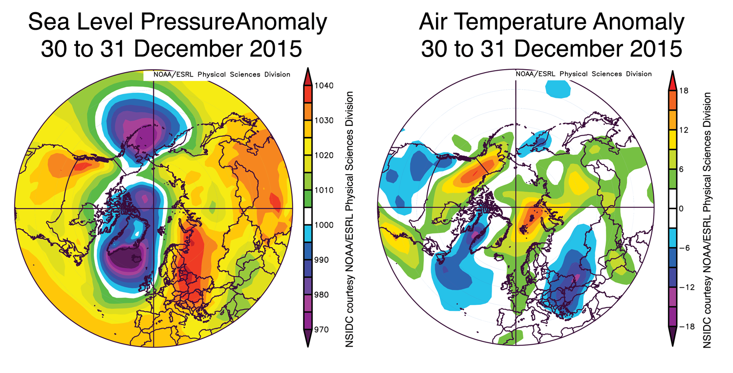
The average ice loss during May 2016 was 61,000 square kilometers (23,600 square miles) per day. This was faster than the 1981 to 2010 long-term average rate of decline of 46,600 square kilometers (18,000 square miles) per day. May air temperatures at the 925 hPa level were 2 to 3 degrees Celsius (4 to 5 degrees Fahrenheit) above the 1981 to 2010 average across most of the Arctic Ocean, with localized higher temperatures in the Chukchi Sea (4 to 5 degrees Celsius or 7 to 9 degrees Fahrenheit) and in the Barents Sea (4 degrees Celsius or 7 degrees Fahrenheit). Air pressure patterns were not particularly unusual, but two areas of southerly winds in northern Europe and Alaska pushed higher than average temperatures into the Arctic Ocean, producing hot spots noted above and generally above-average temperatures across the Arctic. Only over central Siberia were temperatures lower than the 1981 to 2010 average.

May 2016 compared to previous years

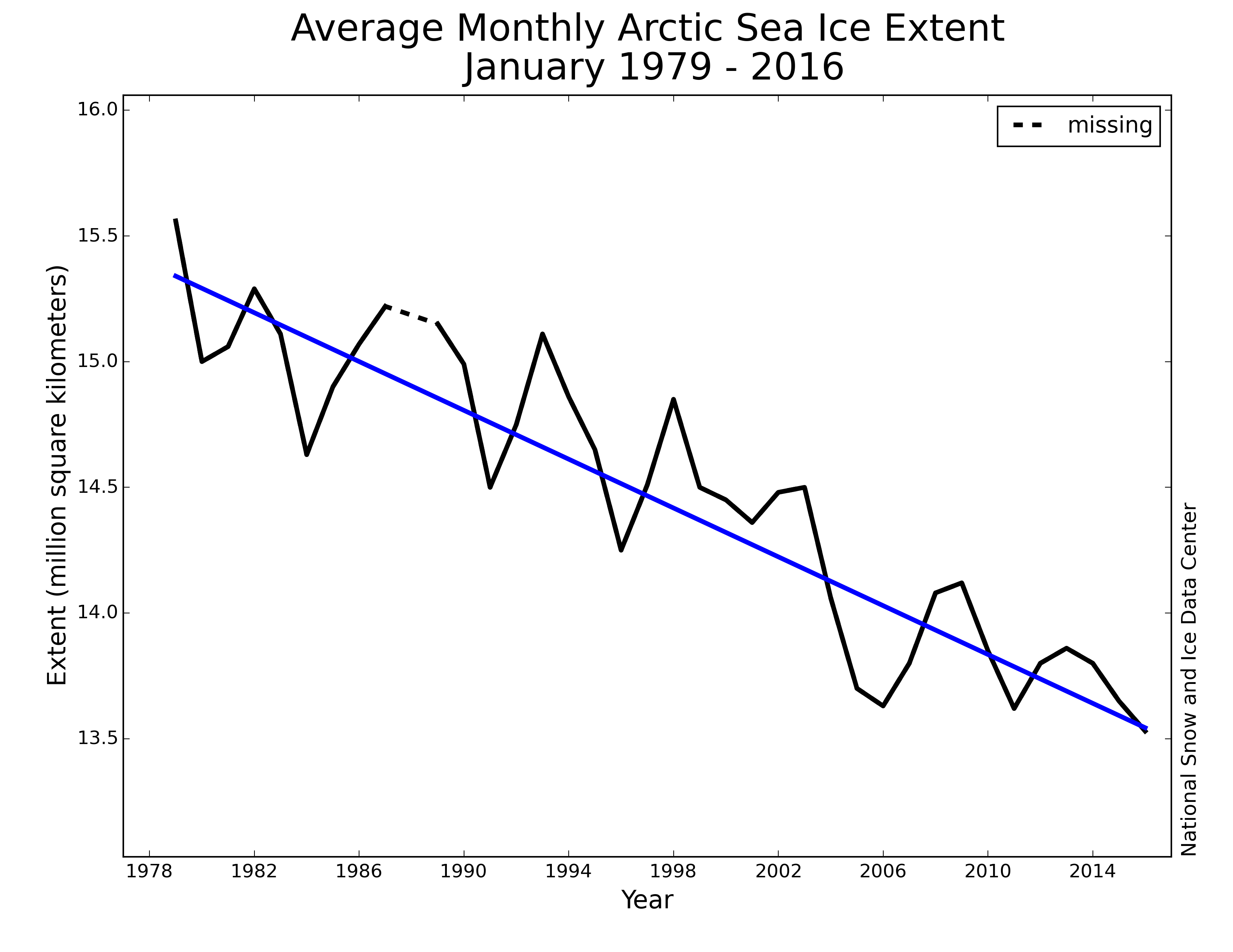
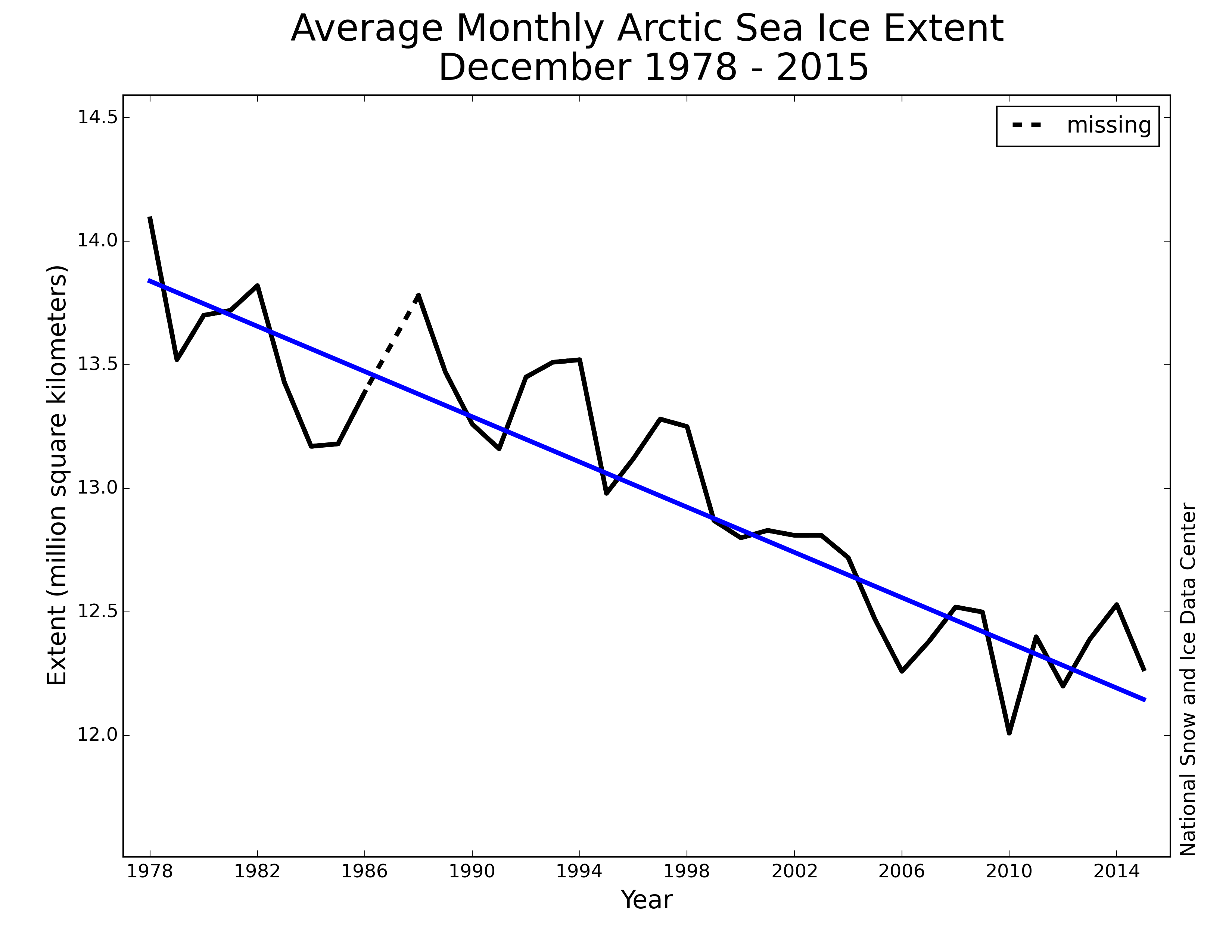
Figure 3. Monthly May Arctic sea ice extent for 1979 to 2016 shows a decline of 2.6 percent per decade. Provisional data. Not a Sea Ice Index product.

Credit: National Snow and Ice Data Center
High-resolution image

Through 2016, the rate of decline for the month of May is 34,000 square kilometers (13,000 square miles) per year, or 2.6 percent per decade.

Thickness in the Beaufort Sea

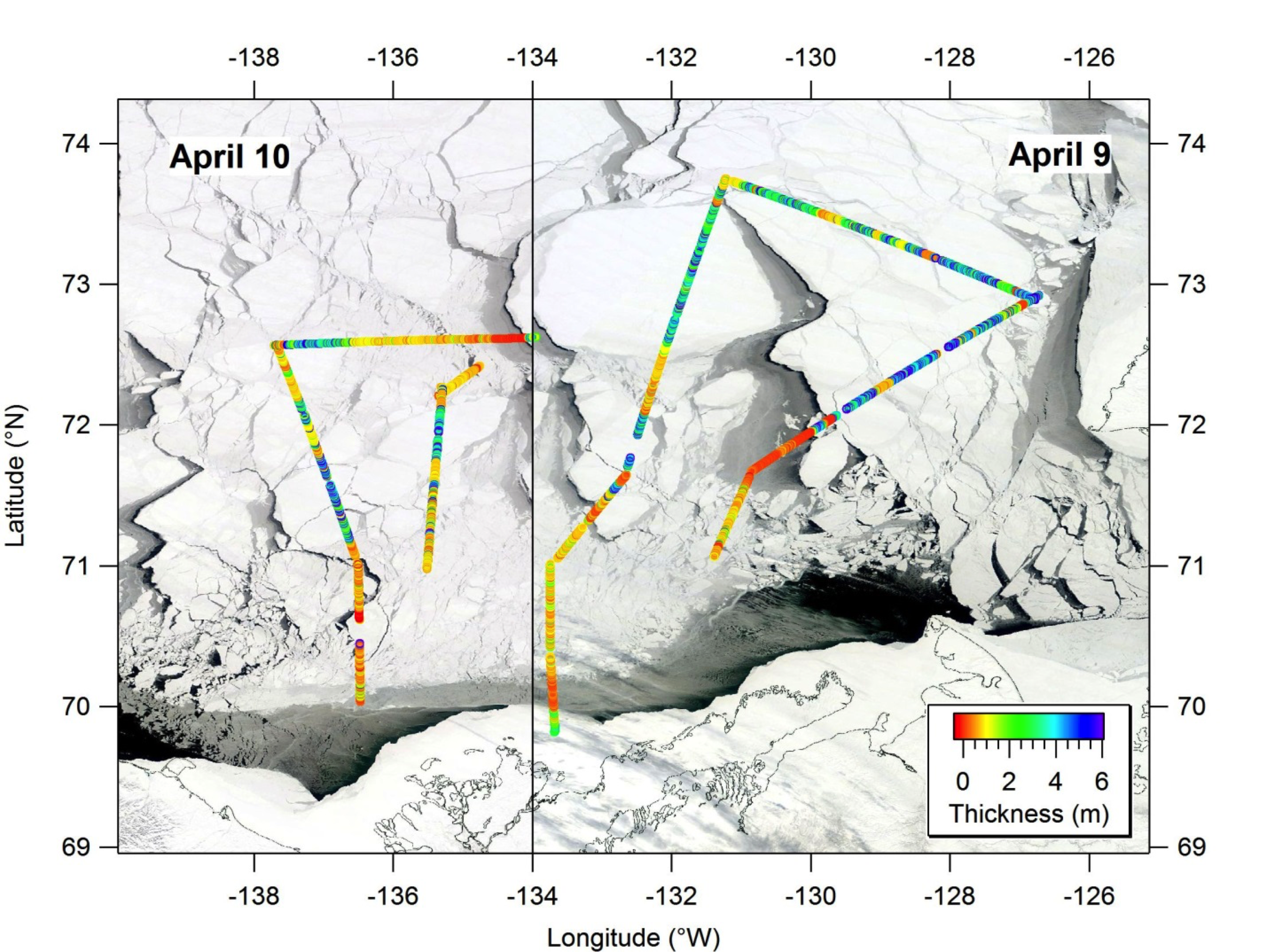
Figure 4a. The image above shows ice thickness measurements in the Beaufort Sea on April 9 and 10, 2016, superimposed on concurrent imagery from the Moderate Resolution Imaging Spectroradiometer (MODIS) sensor on the NASA Terra and Aqua satellites. Short black lines demarcate the boundary between first-year (south) and multiyear (north) regimes.

Credit: C. Haas, York University
High-resolution image

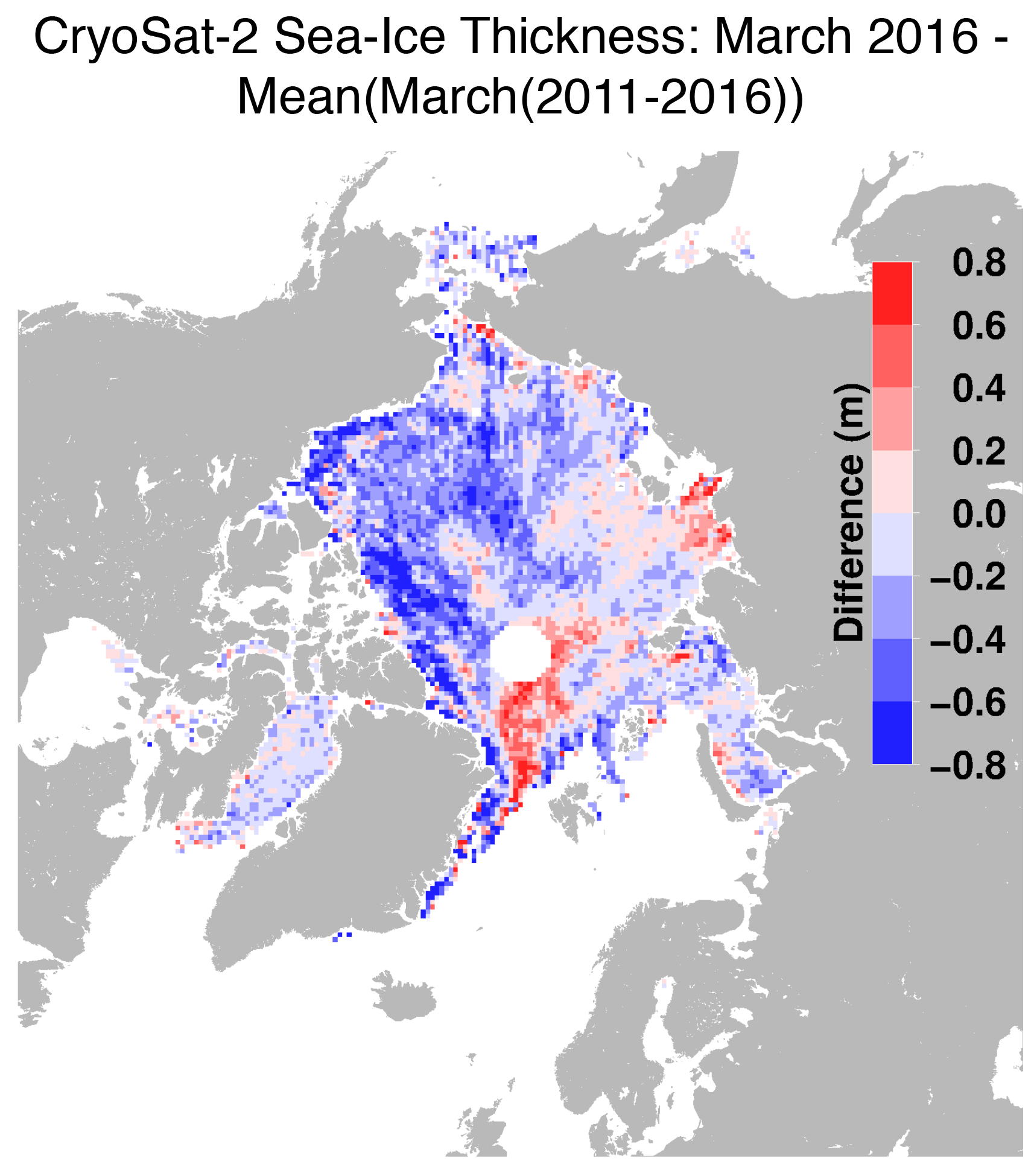
Figure 4b. This figure shows the difference between March ice thickness and the average of March 2011 to 2016. Data are from the European Space Agency’s CryoSat-2 satellite.

Credit: R. Ricker, Helmholtz Centre for Polar and Marine Research, ESA
High-resolution image

Satellite and survey data show that ice thicknesses in parts of the Arctic are similar to those observed in 2015, but that ice thickness over the whole region is thinner compared to the last five years. Ice thickness surveys carried out by York University in early April 2016 show that thicknesses in the Northwest Passage are similar to that in 2015, though there is less multiyear ice in 2016. In the southern Beaufort Sea, the thickness of multiyear ice is also similar to the previous year, but because of strong divergence and export, first-year sea ice is considerably thinner than in 2015, giving rise to expectations of earlier melt out of this thin ice and formation of open water in 2016. Data from the European Space Agency’s CryoSat-2 satellite show that first-year ice in March 2016 is thinner compared to the March 2011 to 2016 average, especially in the Beaufort Sea (20 to 40 centimeters thinner) and the Barents and Kara seas (10 to 30 centimeters thinner). Multiyear ice north of Canada and Greenland is also thinner.

The thinner first year ice may partly explain the early development of open water in the southern Beaufort Sea for this month. The multiyear ice on the other hand may survive and slow down the overall retreat of the ice edge, as it did in 2015 when a band of multiyear ice survived throughout most of the summer. However, the multiyear ice regime this year seems more fragmented and interspersed with thinner first-year ice. When this thinner ice melts, dark open water areas may grow rapidly as energy is absorbed which in turn melts more ice and can accelerate multiyear ice decay.

Fragmented ice in the Beaufort Sea

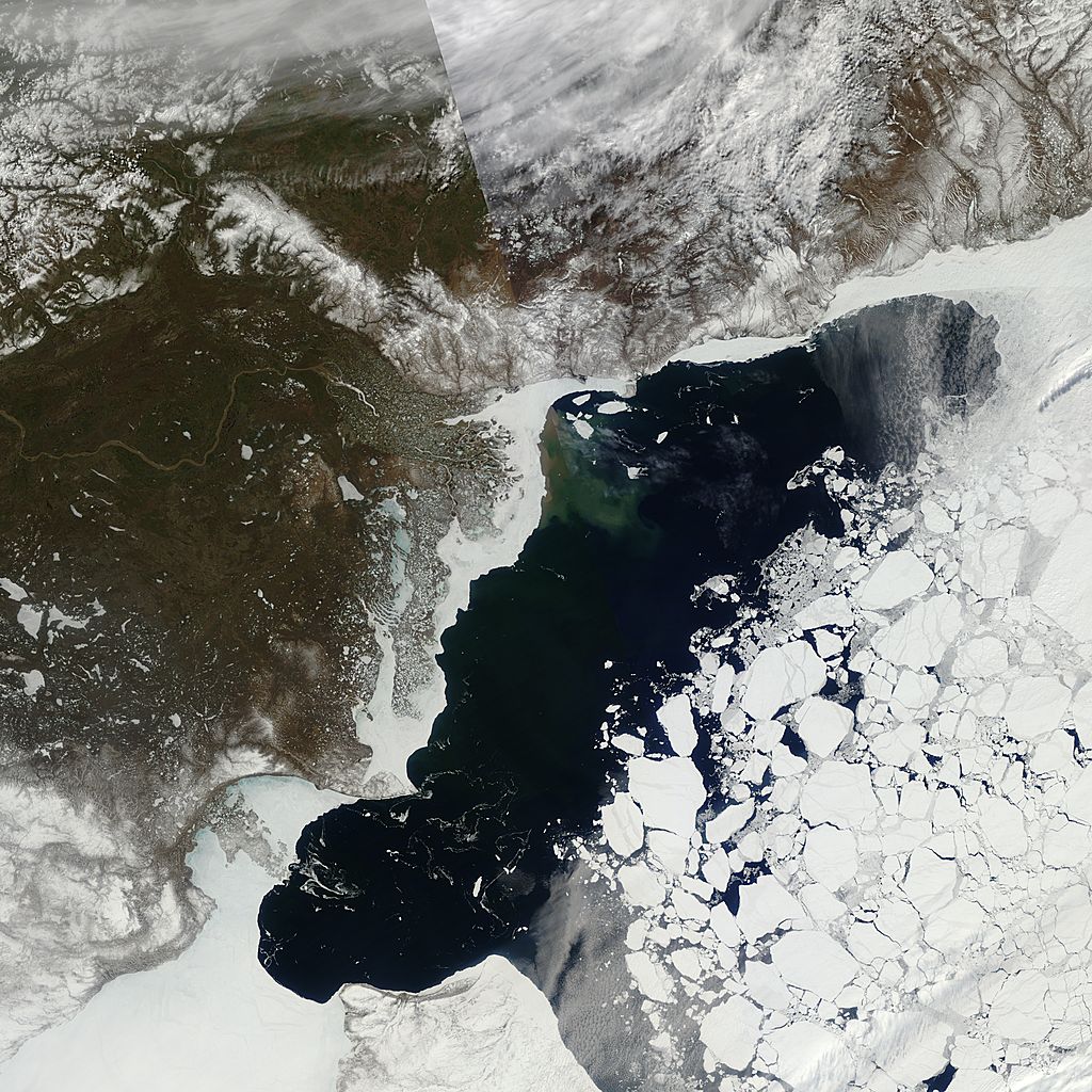
Figure 5. The image above shows a May 21, 2016 view of Arctic sea ice in the Beaufort Sea from the Moderate Resolution Imaging Spectroradiometer (MODIS) sensor.

Credit: Land Atmosphere Near-Real Time Capability for EOS (LANCE) System, NASA/GSFC
High-resolution image

As discussed in last month’s post, a large area in the Beaufort Sea shows a very fragmented ice cover as a result of strong wind-driven divergence throughout the late winter and spring. Figure 5 shows a MODIS visible-band image from May 21, 2016 for the southern Beaufort Sea, illustrating how the fragmentation has led to large multiyear ice floes surrounded by first-year ice and open water. The area of fragmented ice now nearly reaches the pole. While thick, multiyear ice can better survive the summer melt season, the early development of open water allows temperatures in the ocean mixed layer (top 20 meters) to rise, which may enhance lateral ice melt in that region. In summer 2007, early retreat of sea ice from the coasts of Siberia and Alaska, combined with unusual clear skies, led to enhanced melt of thick multiyear ice floes, some recording nearly 3 meters (10 feet) of bottom melt. If atmospheric conditions this summer are as favorable as they were in 2007, some of this multiyear ice may not survive the summer.

Report from the field: Barrow, Alaska

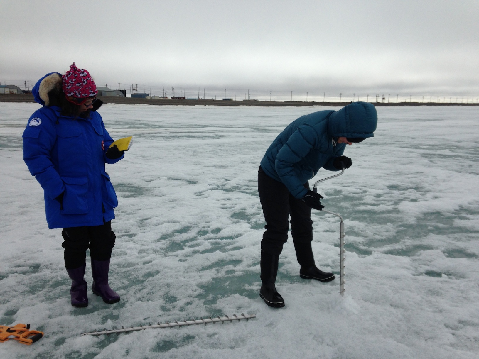
Figure 6a. Researchers use an auger to drill into the sea ice off Barrow, Alaska. After drilling a hole, they would then use a tape measure to record ice thickness.

Credit: W. Meier, NASA
High-resolution image

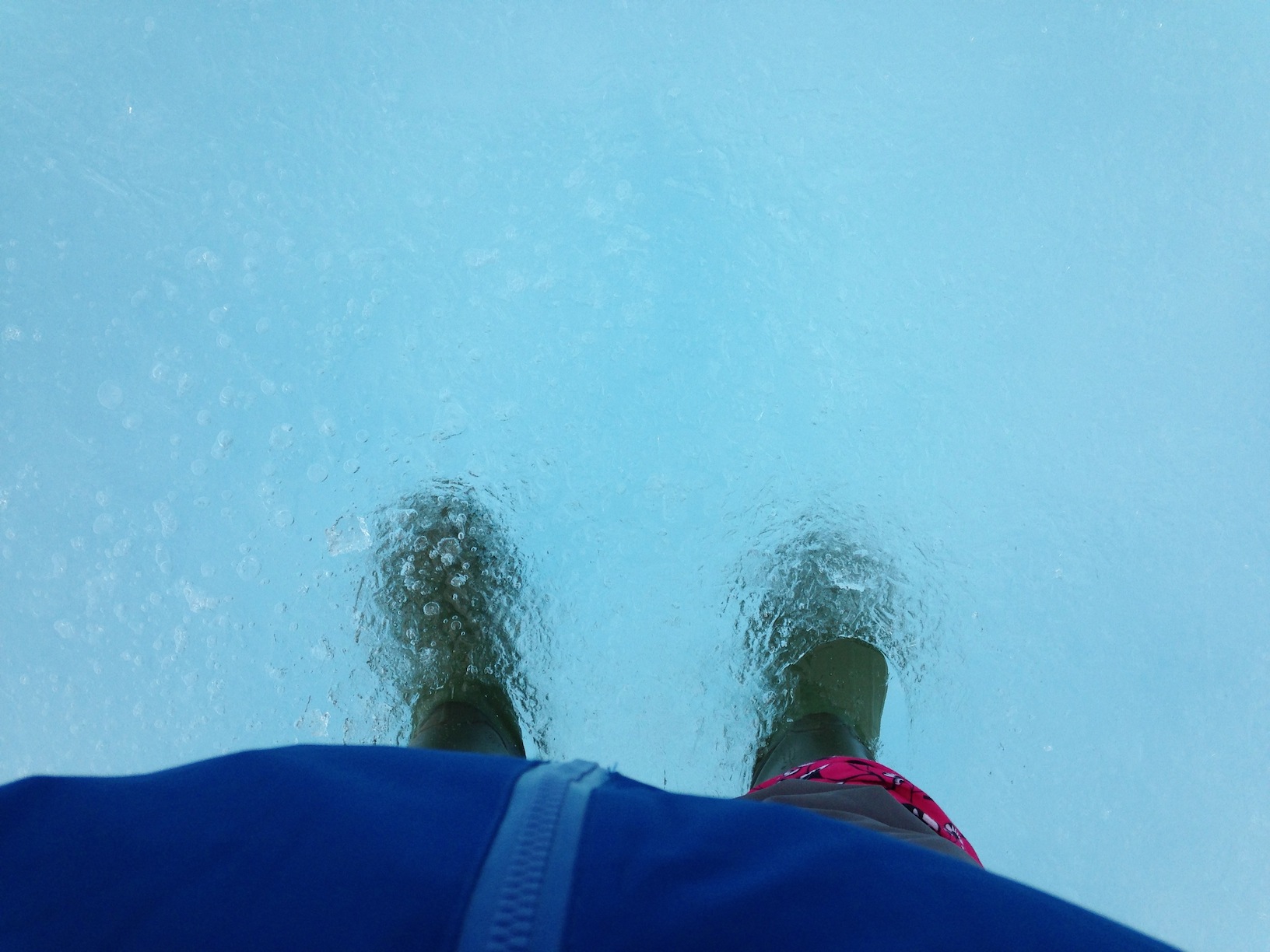
Figure 6b. NASA researcher Walt Meier stands in a melt pond on the sea ice off Barrow, Alaska.

Credit: W. Meier, NASA
High-resolution image

NASA research scientist and NSIDC Arctic Sea Ice Analysis contributor Walt Meier spent the last week in Barrow, Alaska taking part in a National Science Foundation-funded sea ice camp and workshop. The goal was to bring together modelers, remote sensing scientists, and field researchers to understand each other’s work and to develop new ways to collaborate and combine knowledge about the Arctic sea ice system. As part of the camp, groups trudged onto the ice daily to take measurements. They found the ice to be quite thin at 80 to 100 centimeters (31 to 39 inches), compared to an average year when thicknesses would be 140 to 150 centimeters (55 to 59 inches). Melt ponds had already formed, though during cooler days, there was some refreezing as well. The residents of Barrow conveyed that it has been a very unusual winter. Normally, there is quite a bit of onshore wind from the west. This pushes the ice together and grounds pieces to the shallow shelf offshore, which helps stabilize the ice cover. However, this year the winds have been almost always from the east. This keeps the ice near the shore flat and undeformed (which the group observed during the camp) and opens up leads, or areas of open water, at the edge of the fast ice, which is clear in satellite imagery. This westward flow is a part of the larger Beaufort Gyre flow that has dominated the entire Beaufort and Chukchi sea region for much of the winter.

Record low snow

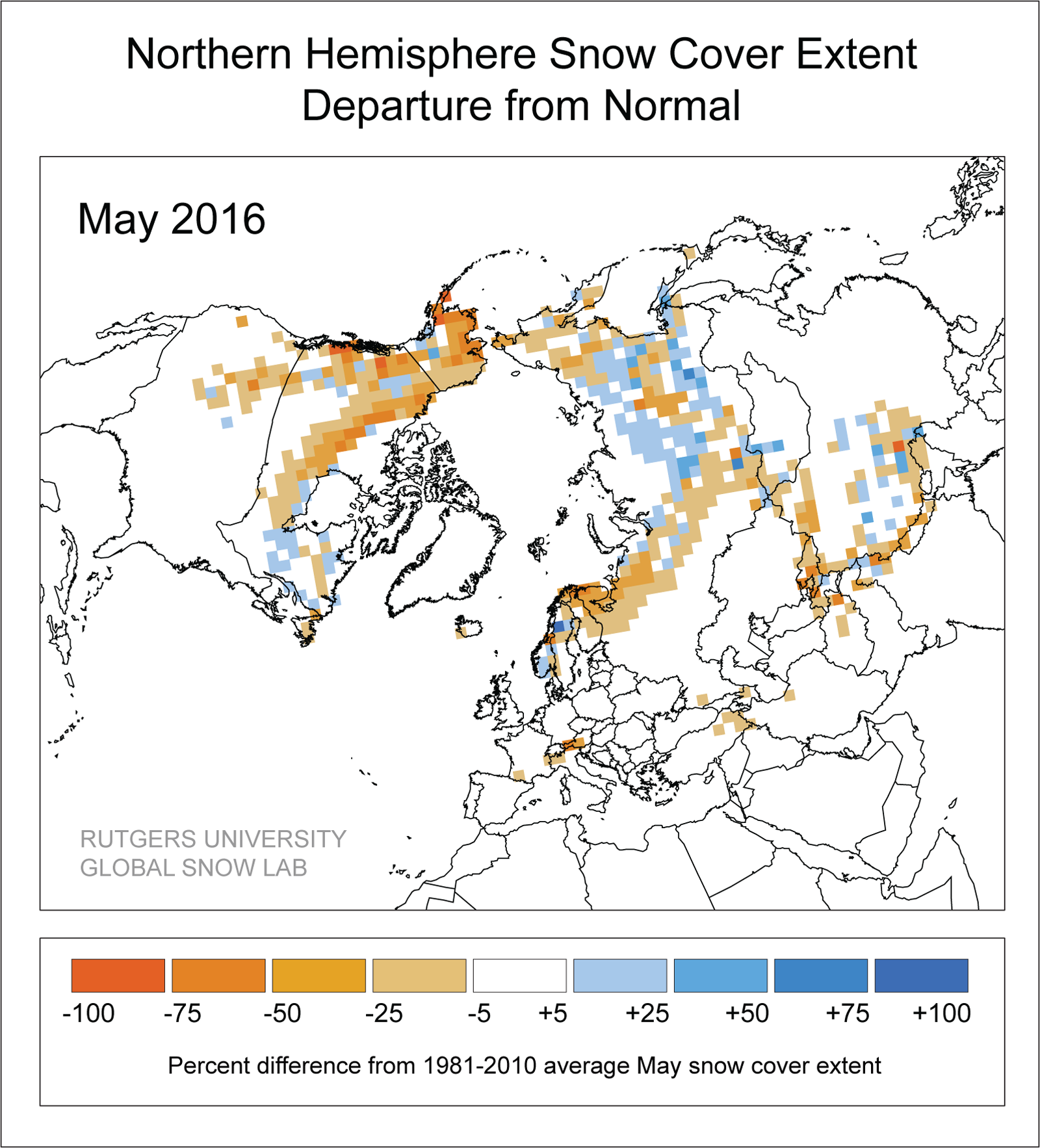
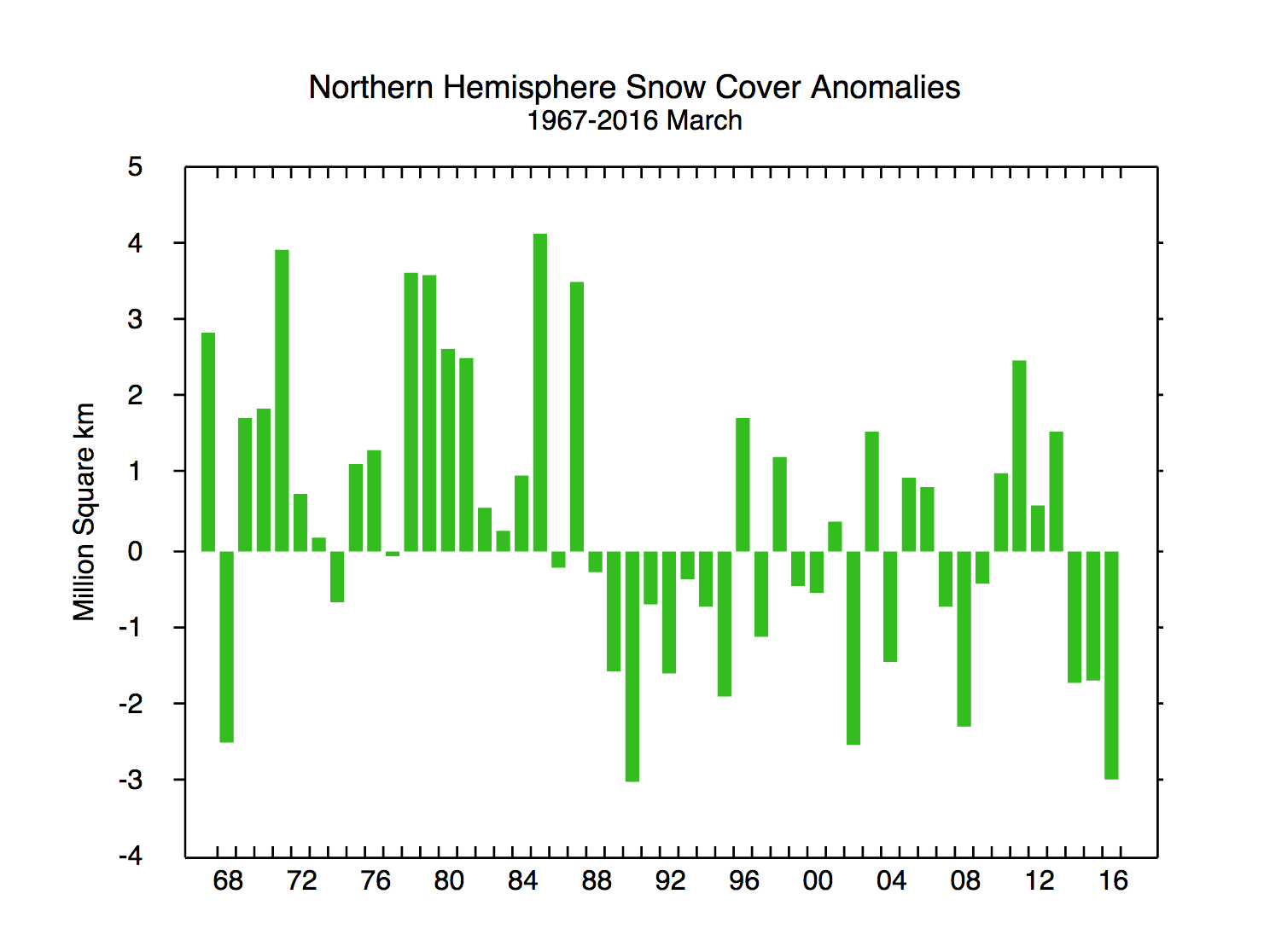
Figure 7. This snow cover anomaly map shows the percent difference between snow cover for May 2016 compared with average snow cover for May from 1981 to 2010. Areas in orange and red indicate lower than usual snow cover, while regions in blue had more snow than average.

Credit: D. Robinson and T. Estilow, Rutgers University Global Snow Lab
High-resolution image

The Northern Hemisphere had exceptionally low snow coverage for both April and May of 2016 and a record low spring (March, April, and May), as reported from 50 years of mapping by Rutgers University’s Global Snow Lab. April’s snow cover was the lowest at 27.91 million square kilometers (10.78 million square miles), and May was the fourth lowest at 16.34 million square kilometers (6.3 million square miles).

The National Oceanic and Atmospheric Administration announced on May 20 that Barrow, Alaska recorded the earliest snowmelt (snow-off date) in 78 years of recorded climate history. Typically snow retreats in late June or early July, but this year the snowmelt began on May 13, ten days earlier than the previous record for that location set in 2002.

Below average sea ice in the Antarctic

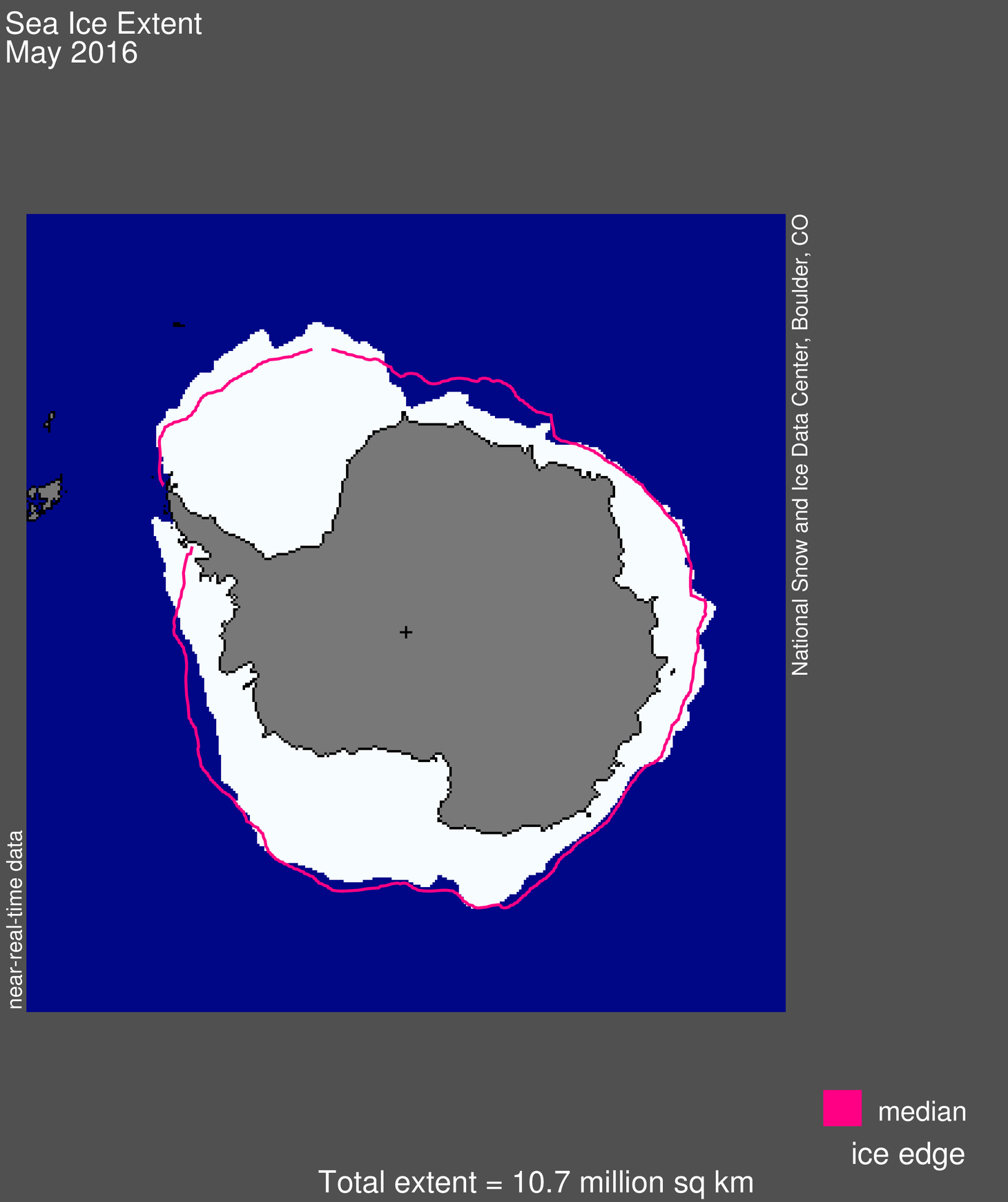
Figure 8a. Antarctic sea ice extent for May 2016 was 10.6 million square kilometers (4.13 million square miles). The magenta line shows the 1981 to 2010 median extent for that month. The black cross indicates the geographic South Pole. Provisional data. Not a Sea Ice Index product.

Credit: National Snow and Ice Data Center
High-resolution image

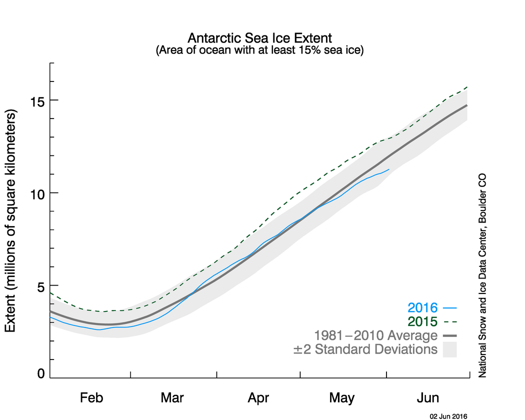
Figure 8b. The graph above shows Antarctic sea ice extent as of June 2, 2016, along with daily ice extent data for 2015. 2016 is shown in blue and 2015 in green. The 1981 to 2010 average is in dark gray. The gray area around the average line shows the two standard deviation range of the data. Sea Ice Index data.

Credit: National Snow and Ice Data Center
High-resolution image

Sea ice extent in the Southern Hemisphere grew fairly slowly in May compared to the average, causing it to dip below the long-term average by the second half of the month. Antarctic sea ice extent for May 2016 averaged 10.70 million square kilometers (4.13 million square miles). This is 90,000 square kilometers (35,000 square miles) below the 1981 to 2010 long-term average of 10.79 million square kilometers (4.17 million square miles). Antarctic sea ice has been trending at near-average to below-average levels since June of 2015. In May 2016, extent was particularly low in the Bellingshausen Sea, Fimbul Ice Shelf area, and Wilkes Land Coast, but well above average in the northwestern Weddell Sea near the Antarctic Peninsula.

References

Haas, C. 2012. Airborne observations of the distribution, thickness, and drift of different sea ice types and extreme ice features in the Canadian Beaufort Sea, Proceedings of the Arctic Technology Conference ATC, Houston, Texas, December 3?5, 2012, Paper No. OTC 23812, 8 pp.

Haas, C., and S. E. L. Howell. 2015. Ice thickness in the Northwest Passage, Geophysical Research Letters, 42, doi:10.1002/2015GL065704.

Perovich, D. K., J. A. Richter-Menge, K. F. Jones and B. Light. 2008. Sunlight, water and ice: Extreme Arctic sea ice melt during the summer of 2007, Geophysical Research Letters, 35, L11501, doi:10.1029/2008GL034007.

NSIDC has obtained data from the DMSP F-18 satellite and is in the process of intercalibrating the F-18 data with F-17 data. Intercalibration addresses differences between the series of sensors, in order to provide a long-term, consistent sea ice record. While this work continues, we are displaying the uncalibrated F-18 data in the daily extent image. The daily time series graph shows F-17 data through March 31, and F-18 data from April 1 forward. Initial evaluation of the uncalibrated F-18 data indicates reasonable agreement with F-17, but the data should be considered provisional and quantitative comparisons with other data should not be done at this time.

Because these are provisional data, the Sea Ice Index has not been updated and continues to display only F-17 data through March 31. We expect to make the F-18 data available in Charctic soon.

For general information on the intercalibration of sensors, see the documentation for Sea Ice Concentrations from Nimbus-7 SMMR and DMSP SSM/I-SSMIS Passive Microwave Data. This documentation will be updated when the intercalibration to F-18 is complete.

For more information on the F-17 satellite sensor issues, see our previous post.

The Defense Meteorological Satellite Program (DMSP) F17 satellite is experiencing continuing issues with its passive microwave sensor. Data from the 37V channel, used to observe sea ice, have been unusable since early April, although the 37H channel used for the Greenland Ice Sheet Today melt area mapping is unaffected. NSIDC is working to bring the DMSP F18 satellite online for its near-real-time source of data for sea ice monitoring. Based on other data sources, sea ice extent remains far below average for the satellite record period, and likely setting record daily lows. The April sea ice decline rate appears to have been slightly faster than average.

Overview of conditions

Figure 1a. Arctic sea ice concentration, in percent concentration, for May 1, 2016 from the Japan Aerospace Exploration Agency (JAXA) satellite Shizuku (GCOM-W1) AMSR2 instrument. Areas of ocean with at least 15% ice concentration are considered ice-covered, when calculating sea ice extent.

Credit: Japan Aerospace Exploration Agency, courtesy University of Bremen
High-resolution image

Figure 1b. The graphs show Arctic sea ice extent as of April 29, 2016, along with ice extent data for previous years. Top, sea ice extent for 2016 from the Japan Aerospace Exploration Agency (JAXA) satellite Shizuku (GCOM-W1) AMSR2 instrument. Bottom, similar plot using the same sensor but a different method and channel, from University of Bremen.

Credit: National Snow and Ice Data Center/JAXA/University of Bremen
High-resolution image

The Arctic Sea Ice News and Analysis reference sea ice product, the Sea Ice Index, will be suspended until a new calibration can be completed for the F18 satellite, which is underway. The Advanced Microwave Scanning Radiometer 2 (AMSR2) instrument flying on Shizuku (GCOM-W1), a satellite operated by the Japan Aerospace Exploration Agency (JAXA), provides data on sea ice extent and rates of change, but because it uses a different sensor and processing algorithm, the extent numbers cannot be directly compared with those from the SMMR-SSM/I-SSMIS instruments record; the AMSR2 algorithm gives extents that differ by several tens of thousands of square kilometers, or a fraction of a percent to a few percent of total sea ice extent.

A look at the Arctic Data archive system at the National Institute of Polar Research in Japan reveals that sea ice since mid-April has remained at record low daily levels as assessed over their archive of sea ice extent, and is approximately 400,000 square kilometers (154,400 square miles) below the previous daily record extents at this time. This is supported by another analysis of sea ice extent produced by the University of Bremen using the same satellite but a different sensor channel. Both assessments of sea ice extent indicate that the April rate of decline for 2016 is slightly faster than the long-term average of their respective archives. Another sea ice monitoring site, The Cryosphere Today, continues to use the DMSP F17 data, and their graphics show evidence of the sensor issues. This site reports sea ice area in its graphical trend, not extent (area of ocean with at least 15% sea ice coverage) as do the other sites and NSIDC. However, the trend and record low daily extents for the second half of April may be interpreted from these data as well.

Conditions in context

Figure 2. Left, sea level pressure for April 2016 relative to average conditions for the same month, 1981 to 2010. Right, air temperature departure from average for April 2016 at the 925 hPa level (approximately 2,500 feet altitude) relative to the same reference period.

Credit: National Snow and Ice Data Center/NOAA ESRL Physical Sciences Division
High-resolution image

April 2016 was quite warm over nearly all of the Arctic Ocean. Air temperatures at the 925 hPa level (about 2,500 feet above the surface) were typically 3 to 5 degrees Celsius (6 to 9 degrees Fahrenheit) above average over the central Arctic Ocean, with larger positive departures compared to average over central Siberia (6 to 8 degrees Celsius, or 11 to 18 degrees Fahrenheit). The sea level pressure pattern featured above average pressures over the Beaufort Sea north of Alaska, and below average pressures over the Aleutians, western Baffin Bay, and Scandinavia. The April 2016 Arctic Oscillation Index transitioned from positive to negative through the month, consistent with the varied patterns of pressure over the Arctic. See our previous discussion of the Arctic Oscillation.

Twist and shout

Figure 3. This series of images from April 1 to 24, 2016 shows recent fracturing and rotation of sea ice near Alaska and the western Canadian Arctic archipelago. Click on the image to see the animation. Images are from the Moderate Resolution Imaging Spectroradiometer (MODIS) instrument via NASA Worldview.

Credit: National Snow and Ice Data Center/NASA Worldview
Play the animation

Using a series of images from the Moderate Resolution Imaging Spectrometer (MODIS) from NASA Worldview, we created a short video showing sea ice drift north of Alaska in the Beaufort Sea. The strong anti-cyclonic (high air pressure) pattern produced surface winds that fractured the ice, twisting it in a clockwise direction and opening the pack ice significantly. Dramatic, similar fracturing of sea ice in the Beaufort Sea has been noted in earlier posts (see March 6, 2013).

Motion in the ocean

Figure 4a. Sea ice age mappings for 2015, Week 36 (at the summer sea ice minimum extent) showing the differences between the old (left) and new (right) processing. The improvements in the new processing have resulted in changes in the ice age mapping.

Credit: National Snow and Ice Data Center, courtesy M. Tschudi, C. Fowler, J. Maslanik, R. Stewart/University of Colorado Boulder; W. Meier/NASA Cryospheric Sciences
High-resolution image
View comparison images for 2011 to 2015

Figure 4b. The graph compares the extent of ice in each age category (in years) for 2015 Week 36, at the time of the sea ice minima, from versions 2 (Old NRT) and 3 (New NRT) of the near-real-time ice age algorithm.

Credit: National Snow and Ice Data Center, courtesy W. Meier/NASA Cryospheric Sciences
High-resolution image

The NSIDC sea ice motion and sea ice age products have recently been updated via a release of Version 3. This version was created by re-running the previous algorithms, and incorporating a few improvements. First, a number of unrealistic AVHRR and buoy velocities that had been noted were removed. Also, a more accurate sea ice mask, based on the same sea ice concentration product used in our sea ice extent analysis, was implemented. Finally, the Version 3 updates include buoy-derived motions in the Arctic through the entire time series (1979 to 2015). Near-real-time processing of provisional ice age data, which are frequently shown here as a first look at ice conditions, has also been updated to include some of the improvements of Version 3, including the incorporation of near-real-time buoy data and NSIDC’s near-real-time sea ice concentration product as the basis for the sea ice mask. As with any near-real-time product, the fields should be considered provisional and are subject to change. Full details of the product changes and the new processing methods are included in the product documentation for Polar Pathfinder Daily 25 km EASE-Grid Sea Ice Motion Vectors, Version 3 and EASE-Grid Sea Ice Age, Version 3.

NSIDC has suspended daily sea ice extent updates until further notice, due to issues with the satellite data used to produce these images. The vertically polarized 37 GHz channel (37V) of the Special Sensor Microwave Imager and Sounder (SSMIS) on the Defense Meteorological Satellite Program (DMSP) F-17 satellite that provides passive microwave brightness temperatures is providing spurious data. The 37V channel is one of the inputs to the sea ice retrieval algorithms, so this is resulting in erroneous estimates of sea ice concentration and extent. The problem was initially seen in data for April 5 and all data since then are unreliable, so we have chosen to remove all of April from NSIDC’s archive.

It is unknown at this time if or when the problem with F-17 can be fixed. In the event that the sensor problem has not been resolved, NSIDC is working to transition to another satellite in the DMSP series. Transitioning to a different satellite will require a careful calibration against the F-17 data to ensure consistency over the long-term time series. While this transition is of high priority, NSIDC has no firm timeline on when it will be able to resume providing the sea ice time series. For background information on the challenges of using data in near-real-time, see the ASINA FAQ, “Do your data undergo quality control?”

Low Arctic sea ice extent for March caps a highly unusual winter in the Arctic, characterized by persistent warmth in the atmosphere that helped to limit ice growth. Above-average influx of ocean heat from the Atlantic and southerly winds helped to keep ice extent especially low in the Barents and Kara seas. Northern Hemisphere snow cover for both February and March was also unusually low

Overview of conditions

Figure 1. Arctic sea ice extent for March 2016 was 14.43 million square kilometers (5.57 million square miles). The magenta line shows the 1981 to 2010 median extent for that month. The black cross indicates the geographic North Pole. Sea Ice Index data. About the data

Credit: National Snow and Ice Data Center
High-resolution image

Sea ice extent reached its seasonal maximum on March 24 of 14.52 million square kilometers (5.607 million square miles), barely beating out February 25, 2015 for the lowest seasonal maximum in the satellite record. Arctic sea ice extent averaged for the entire month of March 2016 was 14.43 million square kilometers (5.57 million square miles), the second lowest in the satellite record. This is 1.09 million square kilometers (421,000 square miles) below the 1981 to 2010 average extent, and 40,000 square kilometers (15,000 square miles) above the record low monthly average for March that occurred in 2015. At the end of the month, extent remained well below average everywhere except in the Labrador Sea, Baffin Bay, and Hudson Bay. Ice extent was especially low in the Barents and Kara seas.

Conditions in context

Figure 2. The graph above shows Arctic sea ice extent as of April 3, 2016, along with daily ice extent data for four previous years. 2015 to 2016 is shown in blue, 2014 to 2015 in green, 2013 to 2014 in orange, 2012 to 2013 in brown, and 2011 to 2012 in purple. The 1981 to 2010 average is in dark gray. The gray area around the average line shows the two standard deviation range of the data. Sea Ice Index data.

Credit: National Snow and Ice Data Center
High-resolution image

Because ice extent typically climbs through the first part of March until it reaches its seasonal maximum and then declines, the daily average ice growth rate for the month is typically quite small and is not a particularly meaningful number. This year’s seasonal maximum, while quite low, also occurred rather late in the month. Very early in the month, extent declined, raising anticipation that an early maximum had been reached. However, after a period of little change, extent slowly rose again, reaching the seasonal maximum on March 24.

March of 2016 saw unusually warm conditions over nearly all of the Arctic Ocean. Air temperatures at the 925 hPa level (about 3,000 feet above the surface) were typically 2 to 4 degrees Celsius (4 to 7 degrees Fahrenheit) above average over the Arctic coastal seas, with larger positive departures compared to average nearer the Pole (4 to 8 degrees Celsius or 7 to 14 degrees Fahrenheit). This was associated with a pattern of above-average sea level pressures centered over the northern Beaufort Sea north of Alaska, and below-average pressures over the Atlantic side of the Arctic, especially pronounced over Baffin Bay and Davis Strait. Through March, the Arctic Oscillation Index bounced between moderate positive and negative values.

March 2016 compared to previous years

Figure 3. Monthly March ice extent for 1979 to 2016 shows a decline of 2.7 percent per decade.

Credit: National Snow and Ice Data Center
High-resolution image

Arctic sea ice extent averaged for March 2016 was the second lowest in the satellite record. Through 2016, the linear rate of decline for March extent is 2.7 percent per decade, or a decline of 42,100 square kilometers (16,200 square miles) per year.

The winter in review

Figure 4. This graph shows differences in Arctic sea ice thickness from December 28, 2015 to January 4, 2016, estimated from the Pan-Arctic Ice Ocean Modeling and Assimilation System (PIOMAS).

Credit: National Snow and Ice Data Center, courtesy PIOMAS
High-resolution image

Figure 5. This figure shows observed (blue columns) and predicted (cyan) winter sea ice area in the Barents Sea. The prediction is based on observed Atlantic heat entering the Barents Sea and the sea ice area the previous year. The predicted sea ice area for this winter (2016) is well below average, and less than that observed for 2015. Anomalously strong southerly winds have also contributed to the very small sea ice area this winter (not shown).

Credit: Ingrid Onarheim/Bjerknes Centre for Climate Research
High-resolution image

Figure 6. This snow cover anomaly map shows the percent difference between snow cover for March 2016, compared with average snow cover for March from 1981 to 2010. Areas in orange and red indicate lower than usual snow cover, while regions in blue had more snow than average.

Credit: National Snow and Ice Data Center, courtesy Rutgers University Global Snow Lab
High-resolution image

Figure 7. This graph shows snow cover extent anomalies in the Northern Hemisphere for March from 1967 to 2016. The anomaly is relative to the 1981 to 2010 average.

Credit: National Snow and Ice Data Center, courtesy Rutgers University Global Snow Lab
High-resolution image

The unusual warmth for March of 2016 continues a pattern of above-average temperatures for most of the Arctic and much of the Northern Hemisphere that has characterized the entire winter. As an exclamation point on the unusual warmth, there was a brief weather event at the very end of December 2015 when air temperatures near the Pole nearly reached the melting point. As we noted in our January post, the event was related to a pulse of warm air moving almost due south to north from the sub-tropical Atlantic to the regions north of Svalbard, an atmospheric river set between broad high and low pressure areas in Europe and the north Atlantic.

The December event also led to higher than average air temperatures over the Kara and Barents seas, reducing the sea ice concentration and causing thinning of the ice that was there. While sea ice normally grows and thickens over winter, the difference in thickness estimated from Pan-Arctic Ice Ocean Modeling and Assimilation System (PIOMAS) shows that between December 28, 2015 and January 4, 2016, sea ice within the Kara and Barents seas thinned by more than 30 centimeters (Figure 4). Thinning also occurred north of Greenland and off the coast of Siberia, while the ice thickened over most of the Arctic Ocean. Higher than average temperatures remained in the region after the weather event had passed, which may have further prevented the ice from growing back. The reasons for the persistent warmth over the entire Arctic this past winter are currently under investigation; a link with the strong El Niño pattern of this winter may be involved.

While the warm atmospheric conditions played a role in the low ice extent for March 2016, the especially low extent that has persisted in the Barents and Kara seas appears to be linked with another heat source—an influx of warm Atlantic waters, entering between Bear Island and Norway (the Barents Sea opening). Ingrid Onarheim from the Bjerknes Centre for Climate Research in Bergen, Norway has been studying this issue and predicted a small sea ice cover in the Barents Sea this winter based on observed Atlantic heat transport to the Barents Sea through April 2015 (Figure 5). In addition to the above-average ocean heat transport, prevailing southerly winds have pushed the sea ice northward since November 2015, bringing in warm air that damps the normally high ocean-air heat loss and favoring ice formation. This likely contributed to the below-average ice conditions in the Arctic this winter. Atlantic heat transport due to near-surface ocean currents reached a long-term maximum in the mid-2000s. Several studies have suggested a more moderate inflow of Atlantic waters may characterize the years ahead, leading to increases in the Barents Sea ice cover in the coming years.

Along with low sea ice extent and above-average temperatures, March of 2016 also saw a very low monthly snow cover extent for the Northern Hemisphere (Figures 6 and 7). Snow cover was low across northern Eurasia, with only minor areas of above-average snow cover in western Turkey, northern Kazakhstan and Mongolia, and easternmost High-Mountain Asia. In North America, snow cover was low across nearly all of the coterminous 48 states in the U.S., despite a series of storms late in the month in the central Rockies and Great Plains. Overall, March 2016 had 37.16 million square kilometers (14.35 million square miles) of snow cover extent, 2.97 million square kilometers (1.15 million square miles) below the 1981 to 2010 average of 40.13 million square kilometers (15.50 million square miles). This makes March 2016 the 49th lowest out of 50 years on record in snow cover extent for the Northern Hemisphere. While April and May could still bring snow to the higher latitudes, we note that low snow cover, similar to low sea ice cover, leads to greater heat absorption by the surface in the Arctic and further warming as we move toward summer.

A younger ice cover

Figure 8. These graphs show Arctic sea ice age from March 4 to 10, 2016. The top graph shows ice age distribution for that week alone and the bottom graph shows ice age distribution for that week from 1985 to 2016.

Credit: NSIDC courtesy University of Colorado Boulder, M. Tschudi, C. Fowler, J. Maslanik, R. Stewart, W. Meier.
High-resolution image

Ice age data for mid-March shows that 70 percent of the sea ice within the Arctic basin consists of first-year ice and only 30 percent is multiyear ice. First-year ice is generally only 1.5 to 2 meters (5 to 6.5 feet) thick. This implies a thinner ice pack as the melt season gets underway. In addition, the oldest ice, or ice at least 5 years or older, is at its smallest level in the satellite record, representing only 3 percent of the total ice cover. Some of this very old ice is found in the western Beaufort Sea and extending towards the Chukchi Sea regions where we have seen large summer ice losses in recent years. Typically this old ice is concentrated north of Greenland and within the Canadian Arctic Archipelago.

Not only is the oldest ice at record low levels, but it it is not recovering. Beginning 2007, we see a strong decline that lasts until 2012 and has not changed much since. If anything it has gone down. In that time we have seen some recovery in younger multiyear ice types: e.g., 2-year ice jumped back up after a one-year minimum, 3-year ice recovered to a lesser degree, and 4-year ice to an even lesser degree. It is not surprising to see some recovery and that first-year ice recovery propagates through time. However, that recovery happens less as the ice gets older, and for 5-year ice and older there is essentially no recovery. The bottom line is that ice no longer survives in the Arctic for very long. It is lasting three to four years tops before melting or advecting out through Fram Strait. This is a big change from the past when much of the ice cover would survive upwards of a decade.

Southern view

Antarctic sea ice grew rapidly in March, rising from below-average daily extents to above-average extents during the month, and increasing by nearly 90,000 square kilometers (35,000 square miles) per day. Sea ice growth was particularly fast in the eastern Ross Sea. Winter temperatures on the continent through the month were near-average overall, but 4 to 6 degrees Celsius (7 to 11 degrees Fahrenheit) below average over the eastern Ross Sea and West Antarctic Ice Sheet.

Arctic sea ice appears to have reached its annual maximum extent on March 24, and is now the lowest maximum in the satellite record, replacing last year’s record low. This year’s maximum extent occurred later than average. A late season surge in ice growth is still possible. NSIDC will post a detailed analysis of the 2015 to 2016 winter sea ice conditions in early April.

Overview of conditions

Figure 1. Arctic sea ice extent for March 24, 2016 was 14.52 million square kilometers (5.607 million square miles). The orange line shows the 1981 to 2010 median extent for that day. The black cross indicates the geographic North Pole. Sea Ice Index data. About the data

Credit: National Snow and Ice Data Center
High-resolution image

On March 24, 2016, Arctic sea ice likely reached its maximum extent for the year, at 14.52 million square kilometers (5.607 million square miles). This year’s maximum ice extent was the lowest in the satellite record, with below-average ice conditions everywhere except in the Labrador Sea, Baffin Bay, and Hudson Bay. The maximum extent is 1.12 million square kilometers (431,000 square miles) below the 1981 to 2010 average of 15.64 million square kilometers (6.04 million square miles) and 13,000 square kilometers (5,000 square miles) below the previous lowest maximum that occurred last year. This year’s maximum occurred twelve days later than the 1981 to 2010 average date of March 12. The date of the maximum has varied considerably over the years, occurring as early as February 24 in 1996 and as late as April 2 in 2010.

Conditions in context

Figure 2. The graph above shows Arctic sea ice extent as of March 27, 2016, along with daily ice extent data for four previous years. 2015 to 2016 is shown in blue, 2014 to 2015 in green, 2013 to 2014 in orange, 2012 to 2013 in brown, and 2011 to 2012 in purple. The 1981 to 2010 average is in dark gray. The gray area around the average line shows the two standard deviation range of the data. Sea Ice Index data.

Credit: National Snow and Ice Data Center
High-resolution image

Sea ice extent was below average throughout the Arctic, except in the Labrador Sea, Baffin Bay, and Hudson Bay. However, it was especially low in the Barents Sea. Below average winter ice conditions in the Kara and Barents seas have been a persistent feature in the last several years, while the Bering Sea has overall seen slightly positive trends towards more sea ice during winter.

Below average sea ice extent is in part a result of higher than average temperatures that have plagued the Arctic all winter. Air temperatures at the 925 hPa level from December 2015 through February 2016 were above average everywhere in the Arctic, with hotspots near the Pole and from the Kara Sea towards Svalbard exceeding 6 Celsius degrees (11 degrees Fahrenheit) above average. These higher than average temperatures continued into March, with air temperatures during the first two weeks reaching 6 degrees Celsius (11 degrees Fahrenheit) above average in a region stretching across the North Pole toward northern Greenland, and up to 12 degrees Celsius (22 degrees Fahrenheit) above average north of Svalbard.

These unusually warm conditions have no doubt played a role in the record low ice extent this winter. Another contributing factor has been a predominance of southerly winds in the Kara and Barents seas that have helped to keep the ice edge northward of its typical position. This area has also seen an influx of warm Atlantic waters from the Norwegian Sea.

There is little correlation between the maximum winter extent and the minimum summer extent—this low maximum does not ensure that this summer will see record low ice conditions. A key factor is the timing of widespread surface melting in the high Arctic. An earlier melt onset is important to the amount of energy absorbed by the ice cover during the summer. If surface melting starts earlier than average, the snow darkens and exposes the ice below earlier, which in turn increases the solar heat input, allowing more ice to melt. With the likelihood that much of the Arctic cover is somewhat thinner due to the warm winter, early surface melting would favor reduced summer ice cover.

Final analysis pending

At the beginning of April, NSIDC scientists will release a full analysis of winter conditions, along with monthly data for March. For more information about the maximum extent and what it means, see the NSIDC Icelights post, the Arctic sea ice maximum.

Arctic sea ice was at a satellite-record low for the second month in a row. The first three weeks of February saw little ice growth, but extent rose during the last week of the month. Arctic sea ice typically reaches its maximum extent for the year in mid to late March.

Overview of conditions

Figure 1. Arctic sea ice extent for February 2016 was 14.22 million square kilometers (5.48 million square miles). The magenta line shows the 1981 to 2010 median extent for that month. The black cross indicates the geographic North Pole. Sea Ice Index data. About the data

Credit: National Snow and Ice Data Center
High-resolution image

Arctic sea ice extent for February averaged 14.22 million square kilometers (5.48 million square miles), the lowest February extent in the satellite record. It is 1.16 million square kilometers (448,000 square miles) below the 1981 to 2010 long-term average of 15.4 million square kilometers (5.94 million square miles) and is 200,000 square kilometers (77,000 square miles) below the previous record low for the month recorded in 2005.

The first three weeks of February saw little ice growth, but extent rose during the last week of the month primarily due to growth in the Sea of Okhotsk (180,000 square kilometers or 70,000 square miles) and to a lesser extent in Baffin Bay (35,000 square kilometers or 13,500 square miles). Extent is presently below average in the Barents and Kara seas, as well as the Bering Sea and the East Greenland Sea. Extent decreased in the Barents and East Greenland seas during the month of February. In other regions, such as the Sea of Okhotsk, Baffin Bay, and the Labrador Sea, ice conditions are near average to slightly above average for this time of year. An exception is the Gulf of St. Lawrence, which remains largely ice free.

In the Antarctic, sea ice reached its minimum extent for the year on February 19, averaging 2.6 million square kilometers (1 million square miles). It is the ninth lowest Antarctic sea ice minimum extent in the satellite record.

Conditions in context

Figure 2a. The graph above shows Arctic sea ice extent as of March 1, 2016, along with daily ice extent data for four previous years. 2015 to 2016 is shown in blue, 2014 to 2015 in green, 2013 to 2014 in orange, 2012 to 2013 in brown, and 2011 to 2012 in purple. The 1981 to 2010 average is in dark gray. The gray area around the average line shows the two standard deviation range of the data. Sea Ice Index data.

Credit: National Snow and Ice Data Center
High-resolution image

Figure 2b. These three images show two-week average Arctic sea ice drift data from January through mid-February derived from the Advanced Microwave Scanning Radiometer 2 (AMSR-2). The image on the left shows the period January 1 to 15, the middle image shows January 14 to 31, and the image on the right shows February 1 to 16.

Credit: Alek Petty/NASA Goddard Space Flight Center/University of Maryland, data from Centre ERS d’Archivage et de Traitement (CERSAT)/French Institute for Exploration (Ifremer)
High-resolution image

NASA and NOAA announced that January 2016 was the ninth straight month of record-breaking high surface temperatures for the globe. In terms of regional patterns, the Arctic stands out, with surface temperatures more than 4 degrees Celsius (7.2 degrees Fahrenheit) above the 1951 to 1980 average. These high temperatures were in part responsible for the record low sea ice extent observed for January. Persistent warmth has continued into February; air temperatures at the 925 hPa level were 6 to 8 degrees Celsius (11 to 14 degrees Fahrenheit) above the 1981 to 2010 average over the central Arctic Ocean near the pole. The rate of ice growth for February was near average at 19,700 square kilometers (7,600 square miles) per day, compared to 20,200 square kilometers (7,800 square miles) per day for the 1981 to 2010 average.

Atmospheric circulation patterns have also favored low sea ice extent, particularly in the Barents and Kara seas. Ice motion drift data derived from the Advanced Microwave Scanning Radiometer 2 (AMSR2) satellite and provided by the Centre ERS d’Archivage et de Traitement (CERSAT) show that since January 1, there has been cyclonic, or counterclockwise, sea ice motion in the Barents Sea helping to keep sea ice from advancing south. During the second half of January, an anti-cyclonic, or clockwise, circulation pattern developed in the Beaufort Sea, which subsequently strengthened and expanded to include most of the Arctic Ocean. This, combined with high pressure over Greenland and low pressure over Spitsbergen, has favored enhanced ice export out of Fram Strait, helping to flush old, thick ice out of the Arctic Ocean, leaving behind thinner ice that is more apt to melt away in summer. Whether this circulation pattern will continue and set the stage for very low September sea ice extent remains to be seen.

February 2016 compared to previous years

Figure 3. Monthly February sea ice extent for 1979 to 2016 shows a decline of 3.0 percent per decade.

Credit: National Snow and Ice Data Center
High-resolution image

February 2016 sea ice extent was the lowest in the satellite record at 14.22 million square kilometers (5.48 million square miles). The linear rate of decline for February is now 3.0 percent per decade.

Record warmth revealed by the AIRS instrument

Figure 4. These two images show February 2016 departures from the 2003 to 2015 average for 925 hPa air temperature (left) and precipitable water (right) as derived from the NASA AIRS instrument.

Credit: Linette Boisvert/NASA Goddard Space Flight Center
High-resolution image

Since 2003, the Atmospheric Infrared Sounder (AIRS) onboard the NASA Aqua satellite has collected daily temperature and humidity profiles globally. Although the record is fairly short, AIRS data can provide insight into recent changes in Arctic climate. February average air temperatures, measured by AIRS at 925 hPa, are around 5 degrees Celsius (9 degrees Fahrenheit) above the 2003 to 2015 average over the Beaufort and Chukchi seas and the central Arctic Ocean. Above-average temperatures are also the rule over the Kara Sea and Northern Siberia (6 degrees Celsius or 11 degrees Fahrenheit above average). Regions with especially higher than average temperatures correspond to regions of low sea ice, demonstrating the role played by heat fluxes from open water areas. For example, the Sea of Okhotsk experienced below-average air temperatures, and also had above-average sea ice extents, whereas the Kara, Barents, and Bering seas and the Gulf of St. Lawrence had higher air temperatures compared to average, which coincides with lower than average sea ice extent.

A similar relationship is seen in the total precipitable water for February 2016. Precipitable water is the amount of water vapor in the atmospheric column totaled from the surface to the top of the troposphere, expressed as kilograms of water per square meter (one kilogram per square meter equals 1 millimeter of water depth). In February, areas with precipitable water between 12 percent (Bering Sea) to 70 percent (Kara Sea) above the 2003 to 2015 February average corresponded to regions with below-average sea ice extent. Water vapor is a greenhouse gas, and with more water vapor in the air, there is a stronger emission of longwave radiation to the surface. Conversely, the observation that above-average amounts of water vapor are found over areas of reduced sea ice extent points to a role of local evaporation, and evaporation is a cooling process that by itself will favor ice growth.

A late freeze-up

Figure 5. This images shows freeze-up anomalies in the Arctic for 2015. Reds indicate areas where freeze-up began later than average and blues indicate freeze-up beginning earlier than average.

Credit: National Snow and Ice Data Center, data provided by J. Miller/T. Markus, NASA Goddard Space Flight Center
High-resolution image

Sea ice reformed or refroze later than average throughout most of the Arctic, especially in the Kara and Barents seas where the freeze-up happened about two months later than average. Ice was also late to form in the Beaufort, Chukchi, East Siberian, and Laptev seas, between ten and forty days later than average. In contrast, the timing of freeze-up over the central Arctic Ocean near the pole was near average, as was also the case in Baffin Bay and parts of Hudson Bay. When freeze-up happens late, the ice has less time to thicken before the melt season starts, leading to a thinner ice cover that is more prone to melting out in summer.

References

NASA Goddard Institute for Space Studies. Global Land-Ocean Temperature Index in 0.01 degrees Celsius. http://data.giss.nasa.gov/gistemp/tabledata_v3/GLB.Ts+dSST.txt.

NASA Goddard Institute for Space Studies. NASA, NOAA Analyses Reveal Record-Shattering Global Warm Temperatures in 2015. http://www.giss.nasa.gov/research/news/20160120.

National Oceanic and Atmospheric Administration. Global Analysis – January 2016. https://www.ncdc.noaa.gov/sotc/global/201601.

January Arctic sea ice extent was the lowest in the satellite record, attended by unusually high air temperatures over the Arctic Ocean and a strong negative phase of the Arctic Oscillation (AO) for the first three weeks of the month. Meanwhile in the Antarctic, this year’s extent was lower than average for January, in contrast to the record high extents in January 2015.

Overview of conditions

Figure 1. Arctic sea ice extent for January 2016 was 13.53 million square kilometers (5.2 million square miles). The magenta line shows the 1981 to 2010 median extent for that month. The black cross indicates the geographic North Pole. Sea Ice Index data. About the data

Credit: National Snow and Ice Data Center
High-resolution image

Arctic sea ice extent during January averaged 13.53 million square kilometers (5.2 million square miles), which is 1.04 million square kilometers (402,000 square miles) below the 1981 to 2010 average. This was the lowest January extent in the satellite record, 90,000 square kilometers (35,000 square miles) below the previous record January low that occurred in 2011. This was largely driven by unusually low ice coverage in the Barents Sea, Kara Sea, and the East Greenland Sea on the Atlantic side, and below average conditions in the Bering Sea and Sea of Okhotsk. Ice conditions were near average in Baffin Bay, the Labrador Sea and Hudson Bay. There was also less ice than usual in the Gulf of St. Lawrence, an important habitat for harp seals.

Conditions in context

Figure 2a. The graph above shows Arctic sea ice extent as of February 3, 2016, along with daily ice extent data for four previous years. 2015 to 2016 is shown in blue, 2014 to 2015 in green, 2013 to 2014 in orange, 2012 to 2011 in brown, and 2011 to 2012 in purple. The 1981 to 2010 average is in dark gray. The gray area around the average line shows the two standard deviation range of the data. Sea Ice Index data.

Credit: National Snow and Ice Data Center
High-resolution image

Figure 2b. These graphs show average sea level pressure and air temperature anomalies at 925 millibars (about 3,000 feet above sea level) for January 2016.

Credit: National Snow and Ice Data Center, courtesy NOAA Earth System Research Laboratory Physical Sciences Division
High-resolution image

January 2016 was a remarkably warm month. Air temperatures at the 925 hPa level were more than 6 degrees Celsius (13 degrees Fahrenheit) above average across most of the Arctic Ocean. These unusually high air temperatures are likely related to the behavior of the AO. While the AO was in a positive phase for most of the autumn and early winter, it turned strongly negative beginning in January. By mid-January, the index reached nearly -5 sigma or five standard deviations below average. The AO then shifted back to positive during the last week of January. (See the graph at the NOAA Climate Prediction Web site.)

The sea level pressure pattern during January, which featured higher than average pressure over northern central Siberia into the Barents and Kara sea regions, and lower than average pressure in the northern North Pacific and northern North Atlantic regions, is fairly typical of the negative phase of the AO. Much of the focus by climate scientists this winter has been on the strong El Niño. However, in the Arctic, the AO is a bigger player and its influence often spills out into the mid-latitudes during winter by allowing cold air outbreaks. How the AO and El Niño may be linked remains an active area of research.

January 2016 compared to previous years

Figure 3. Monthly January ice extent for 1979 to 2016 shows a decline of 3.2% per decade.

Credit: National Snow and Ice Data Center
High-resolution image

The monthly average January 2016 sea ice extent was the lowest in the satellite record, 90,000 square kilometers (35,000 square miles) below the previous record low in 2011. The next lowest extent was in 2006. Interestingly, while 2006 and 2011 did not reach record summer lows, they both preceded years that did, though this may well be simply coincidence.

The trend for January is now -3.2% per decade. January 2016 continues a streak that began in 2005 where every January monthly extent has been less than 14.25 million square kilometers (5.50 million square miles). In contrast, before 2005 (1979 through 2004), every January extent was above 14.25 million square kilometers.

Predicting decadal trends in Arctic winter sea ice cover

Figure 4. The map shows areas of the Arctic where sea ice models predicted ice gain and loss for 2007 to 2017

Credit: S. Yeager et al.
High-resolution image

Observations show an increase in the rate of winter sea ice loss in the North Atlantic sector of the Arctic up until the late 1990s followed by a slowdown in more recent years. The observed trend over the period 2005 to 2015 is actually positive (a tendency for more ice). In a paper recently published in Geophysical Research Letters, scientists at the National Center for Atmospheric Research (NCAR) show that the Community Earth System Model (CESM) was able to predict this period of winter ice growth in the North Atlantic. The study further suggests that in the near future, sea ice extent in this part of the Arctic is likely to remain steady or even increase (Figure 4). The ability to predict the winter sea ice extent in this region is related to the ability of the model to capture the observed variability in the Atlantic Meridional Overturning Circulation (MOC), an ocean circulation pattern that brings warm surface waters from the tropics towards the Arctic. When the MOC is strong, more warm water is brought towards the North Atlantic sector of the Arctic, helping to reduce the winter ice cover. When it is weak, less warm water enters the region and the ice extends further south. However, while there is an indication that the MOC may be weakening, this winter so far has seen considerably less ice than average in the North Atlantic sector.

References

Yeager, S. G., A. R. Karspeck, and G. Danabasoglu. 2015. Predicted slowdown in the rate of Atlantic sea ice loss. Geophysical Research Letters, 42, 10,704–10,713, doi:10.1002/2015GL065364.

Correction

On February 8, 2016, a reader called our attention to contradictory sentences in our post. We have corrected the erroneous sentence in the section January 2016 compared to previous years. The sentence used to read “The monthly average January 2016 sea ice extent was the lowest in the satellite record, 110,000 square kilometers (42,500 square miles) less than the previous record low in 2011.” We’ve corrected it to “The monthly average January 2016 sea ice extent was the lowest in the satellite record, 90,000 square kilometers (35,000 square miles) below the previous record low in 2011.” as stated in the section Overview of conditions.

December ended with Arctic sea ice extent tracking between one and two standard deviations below average, as it did throughout the fall. This caps a year that saw the lowest sea ice maximum in February and the fourth lowest minimum in September. In Antarctica, December sea ice extent was slightly above average but far below the exceptionally large ice extents recorded for December 2013 and 2014. A slow-down in the rate of Antarctic sea ice growth in July was followed by near-average extents in the subsequent months. The first week of 2016 has seen very slow ice growth in the Arctic.

Overview of conditions

Figure 1. Arctic sea ice extent for December 2015 was 12.3 million square kilometers (4.74 million square miles). The magenta line shows the 1981 to 2010 median extent for that month. The black cross indicates the geographic North Pole. Sea Ice Index data. About the data

Credit: National Snow and Ice Data Center
High-resolution image

Sea ice extent for December 2015 averaged 12.3 million square kilometers (4.74 million square miles), the fourth lowest December extent in the satellite record. This is 780,000 square kilometers (301,000 square miles) below the 1981 to 2010 average for the month, and 260,000 square kilometers (100,000 square miles) above the record low for December recorded in the year 2010. The rate of sea ice growth slowed slightly through the month and nearly ceased advancing in the first days of the new year, perhaps related to a period of unusual warmth (see below). The ice is currently tracking near two standard deviations below the 1981 to 2010 long-term average. Sea ice extent is well below average in the Bering, Okhotsk, and Barents seas, partly balanced by slightly above average extent in Baffin Bay.

Conditions in context

Figure 2. The graph above shows Arctic sea ice extent as of January 5, 2016, along with daily ice extent data for four previous years. 2015 to 2016 is shown in blue, 2014 to 2015 in green, 2013 to 2014 in orange, 2012 to 2013 in brown, and 2011 to 2012 in purple. The 1981 to 2010 average is in dark gray. The gray area around the average line shows the two standard deviation range of the data. Sea Ice Index data.

Credit: National Snow and Ice Data Center
High-resolution image

Figure 2b. These graphs show average sea level pressure and air temperature anomalies at 925 millibars (about 3,000 feet above sea level) for December 2015.

Credit: NSIDC courtesy NOAA Earth System Research Laboratory Physical Sciences Division
High-resolution image

Arctic sea ice growth for December averaged 65,000 square kilometers (25,000 square miles) per day compared to the long-term average of 64,000 square kilometers (24,700 square miles) per day. Cool conditions at the 925 hPa level (2 to 4 degrees Celsius or 4 to 7 degrees Fahrenheit below average) existed in Baffin Bay, the Alaskan North Slope, and parts of eastern Siberia. A broad area of Europe and western Russia, including the northern Barents Sea, saw temperatures as much as 4 to 8 degrees Celsius (7 degrees to 14 degrees Fahrenheit) above average at the 925 hPa level. Conditions were also fairly warm over the central Arctic Ocean, north of the Canadian Arctic Archipelago. Sea level pressure was below average over much of the Arctic, especially from the northern North Atlantic to the Barents Sea and central Russia, and from the Bering Sea and south along the Canadian Pacific coast (7.5 to 12 millibars below average). This is consistent with the positive phase of the Arctic Oscillation through most of the month, a pattern that has persisted since the end of October.

December 2015 compared to previous Decembers

Figure 3. Monthly December ice extent for 1979 to 2015 shows a decline of 3.4% per decade.

Credit: National Snow and Ice Data Center
High-resolution image

Arctic sea ice extent averaged for December 2015 was the fourth lowest in the satellite record. Through 2015, the linear rate of decline for December extent is 3.4% per decade, or -44,200 square kilometers (-17,000 miles) per year.

2015 in review

The year will be remembered for three major events in sea ice extent: the lowest Arctic maximum in the satellite record, the fourth lowest Arctic minimum in the satellite record, and a return to average levels for Antarctic sea ice extent after more than two years of record and near-record highs.

The record-low Arctic maximum occurred on February 25, 2015 and was among the earliest seasonal maxima in the 37-year satellite record. It was likely a result of very warm conditions in the Sea of Okhotsk and the Barents Sea (4 degrees Celsius or 7 degrees Fahrenheit above average), and low ice extent in the Bering Sea in March (when the maximum would more typically occur). These climate conditions were related to an unusual jet stream pattern as discussed in our April 7, 2015 post.

The fourth lowest Arctic minimum occurred on September 11, 2015 and was likely a consequence of very warm conditions in July and an increasingly young and thin ice cover. The thinner ice is consistent with a tendency in recent years for large polynyas that appear in the Beaufort and Chukchi seas in late summer. Although measurements by the CryoSat-2 satellite indicated that Arctic sea ice was thicker in 2015 compared to pre-2012 thicknesses, the ice behaved as though it was still quite thin.

From February 2013 through June 2015, Antarctic sea ice was at record or near-record daily extents. Antarctic sea ice set consecutive record winter maxima in 2012, 2013 and 2014. (Contrary to 2013 and 2014, autumn and spring conditions in 2012 were near-average.) But during this year’s austral mid-winter period, Antarctic sea ice growth slowed. Since then, extent in the Southern Hemisphere has generally been slightly above average. Climate effects from the building El Niño likely caused the shift during austral mid-winter. A strong El Niño is associated with a change in the position and strength of a major low pressure pattern near West Antarctica, called the Amundsen Sea Low. Weakening of the Amundsen Sea Low, and related impacts elsewhere around the ice edge in Antarctica, tend to reduce ice extent in the Ross Sea, eastern Weddell Sea, and elsewhere around Antarctica except near the Antarctic Peninsula.

The longer view

Figure 4. This graph shows sea ice concentration trends in the Arctic and the Antarctic for March to September for the years 1979 to 2015. Sea Ice Index data. About the data

Credit: National Snow and Ice Data Center
High-resolution image

The satellite passive microwave record for sea ice now spans more than 37 years. As we have documented, clear downward trends characterize Arctic sea ice extent and concentration in all months, while somewhat less emphatic upward trends characterize Antarctic sea ice extent and concentration. A look at the geographic distribution of trends for the seasonal maximum and minimum periods provides insight into how the polar regions are changing. During the Arctic maximum, declines in extent and concentration are pronounced in the Barents Sea and Sea of Okhotsk, but ice cover has increased slightly in the Bering Sea. During the Arctic summer minimum, all areas show negative trends.

Antarctica presents a more mixed picture. During the Antarctic summer minimum, ice cover is increasing around much of the coastline from the Weddell Sea eastward to the western Ross Sea, but is declining sharply in the eastern Ross, Amundsen, and southern Bellingshausen seas. Winter ice cover in Antarctica is characterized by increases in the northern Ross Sea and the Indian Ocean sectors, and decreases in the northwestern Weddell Sea and the region south of Australia.

Ringing in the New Year with a brief polar heat wave

Figure 5. These graphs show average sea level pressure and air temperature anomalies at 925 millibars (about 3,000 feet above sea level) for 30 and 31 December, 2015. The graphs are the average of two days, so the extremes in air pressure and temperature during this period are not shown.

Credit: NSIDC courtesy NOAA Earth System Research Laboratory Physical Sciences Division
High-resolution image

An exceptional weather event during the last days of the year brought a heat wave with surface air temperatures up to 23 degrees Celsius (50 degrees Fahrenheit) above average in the far north, and a brief period when surface temperatures at the North Pole approached or perhaps even exceeded the freezing mark. A temperature of +0.7 degrees Celsius was briefly recorded by a buoy weather station near the North Pole on December 30, 2015. The event was linked to the combination of a very strong low pressure system near Iceland and a somewhat less intense low pressure system located near the North Pole. This was associated with an amplified trough at 500 hPa over the northern North Atlantic and a pronounced ridge of high pressure at 500 hPa to the east over central Europe, extending into the Kara Sea. This created a strong, deep inflow of warm, moist air into the Arctic Ocean’s high latitudes. The low near Iceland strengthened rapidly in the last days of December, reaching a minimum pressure of 935 millibars, equivalent to a hurricane. While the event was remarkable and may account for the slow ice growth during the first few days of January 2016, it was short lived and is unlikely to have any long-term effects on the sea ice cover.

Further reading

Tilling, R. L., A. Ridout, A. Shepherd, D. J. Wingham. 2015. Increased Arctic sea ice volume after anomalously low melting in 2013. Nature Geoscience 8, 643–646, doi:10.1038/ngeo2489.

Thompson, A. “What happened to the Polar Vortex?” ClimateCentral.com. http://www.climatecentral.org/news/what-happened-to-the-polar-vortex-19866?