Arctic sea ice extent maintained a steady, near-average pace of retreat through the first half of August, making it highly unlikely that a new record low minimum will be reached this year. Nevertheless, there are extensive areas of low concentration ice, even in regions close to the North Pole, atmospheric pressure and temperature patterns this summer have differed markedly from those experienced in 2012; cooler than average conditions have prevailed over much of the Arctic Ocean. By contrast, Antarctic sea ice is near a record maximum extent for mid-August.

Overview of conditions

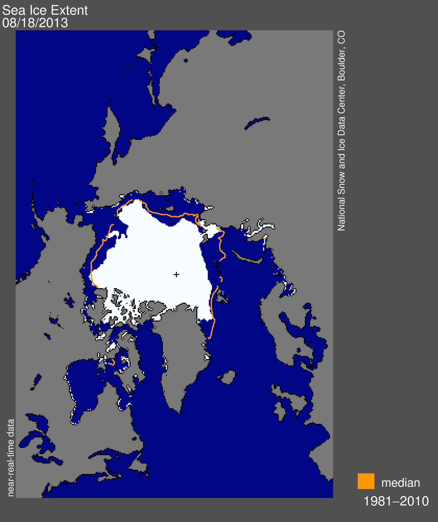
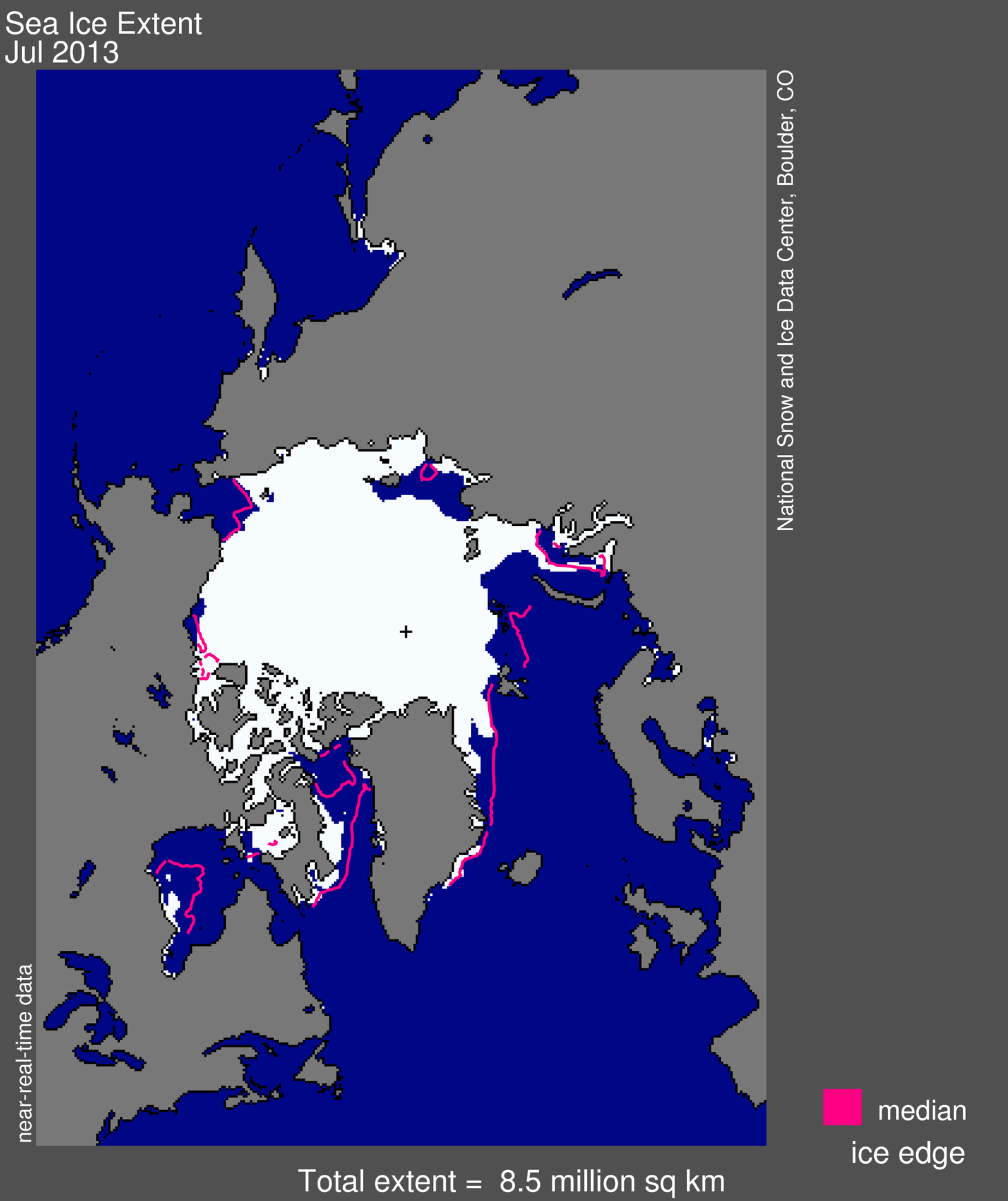
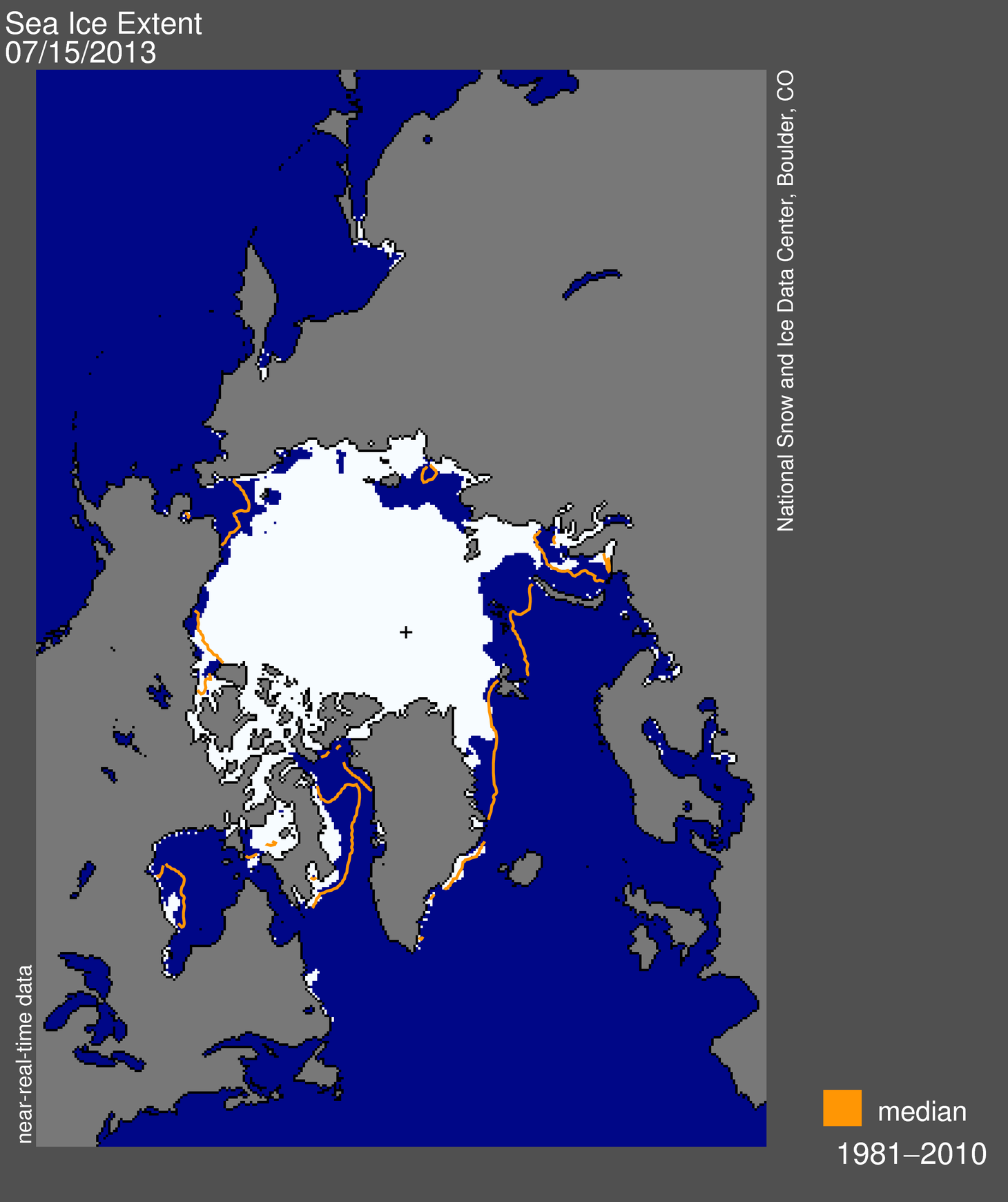
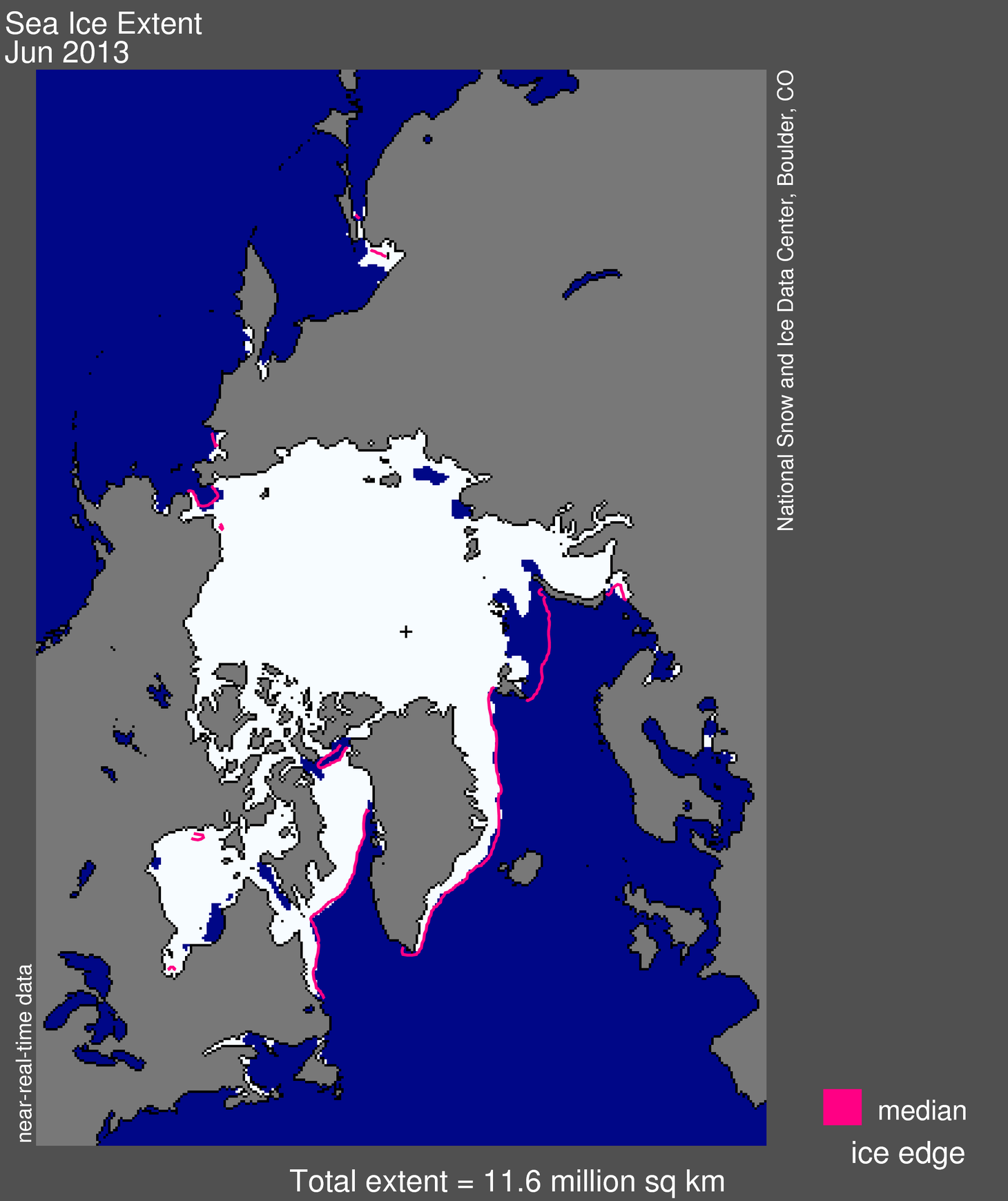
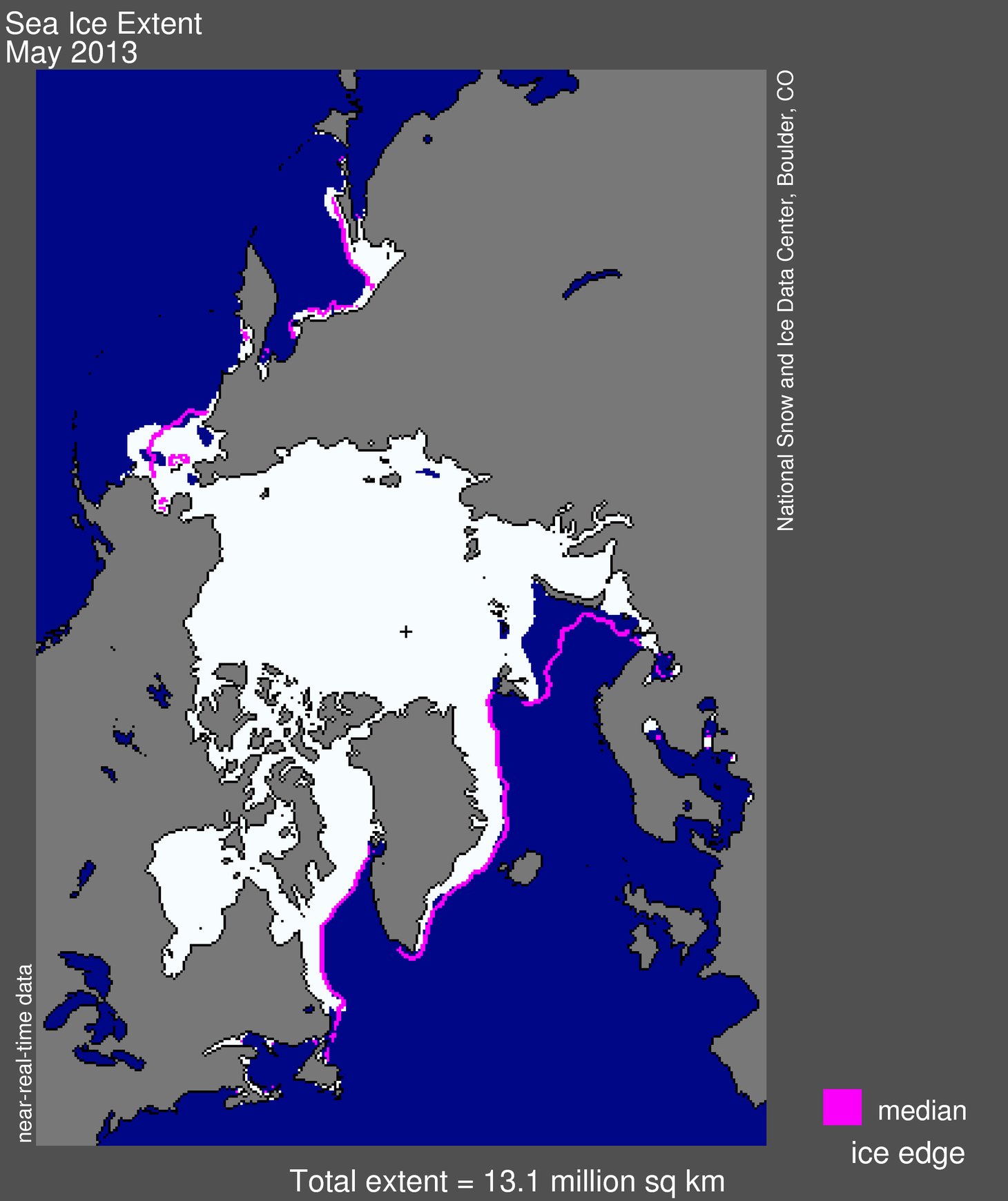
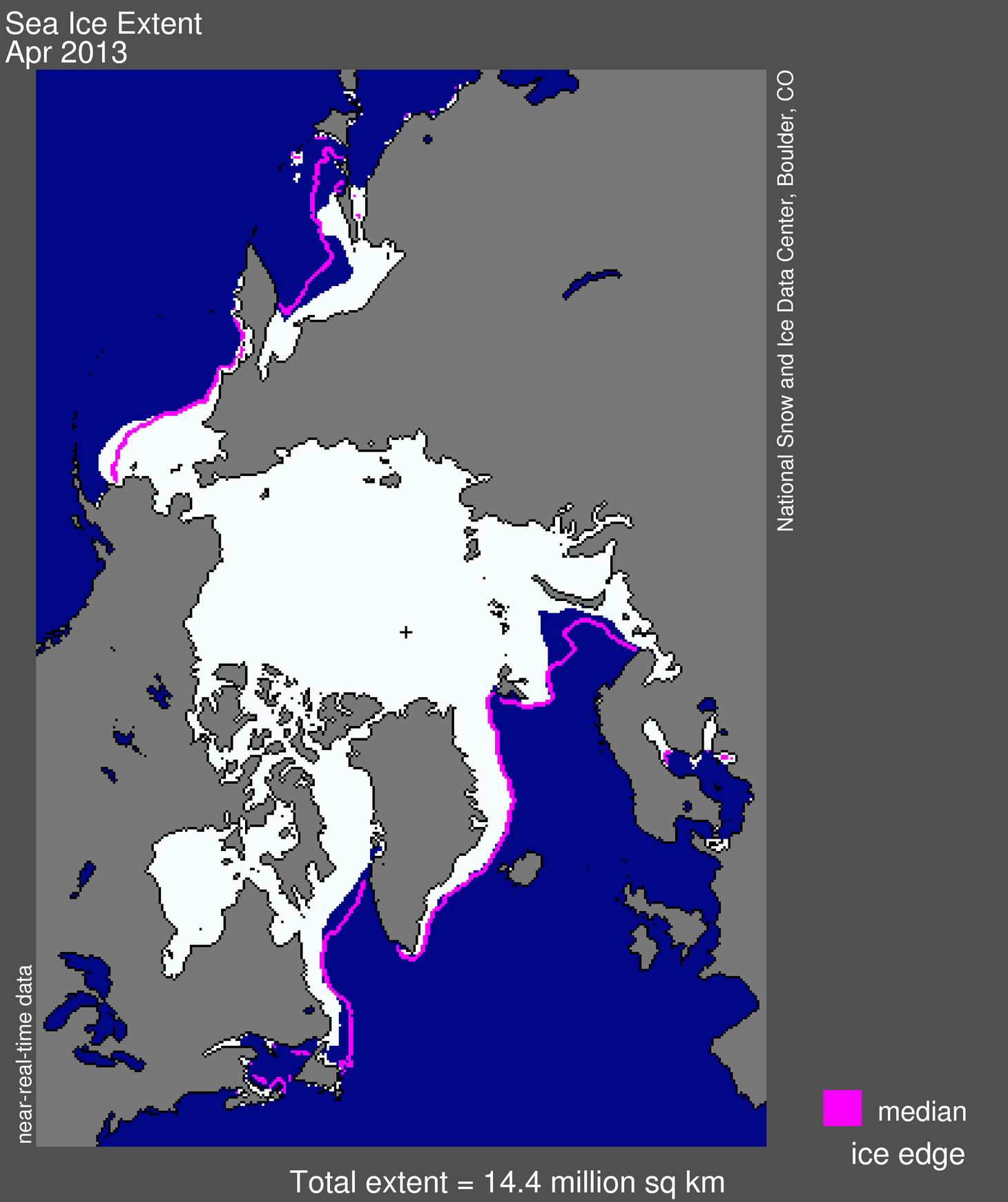
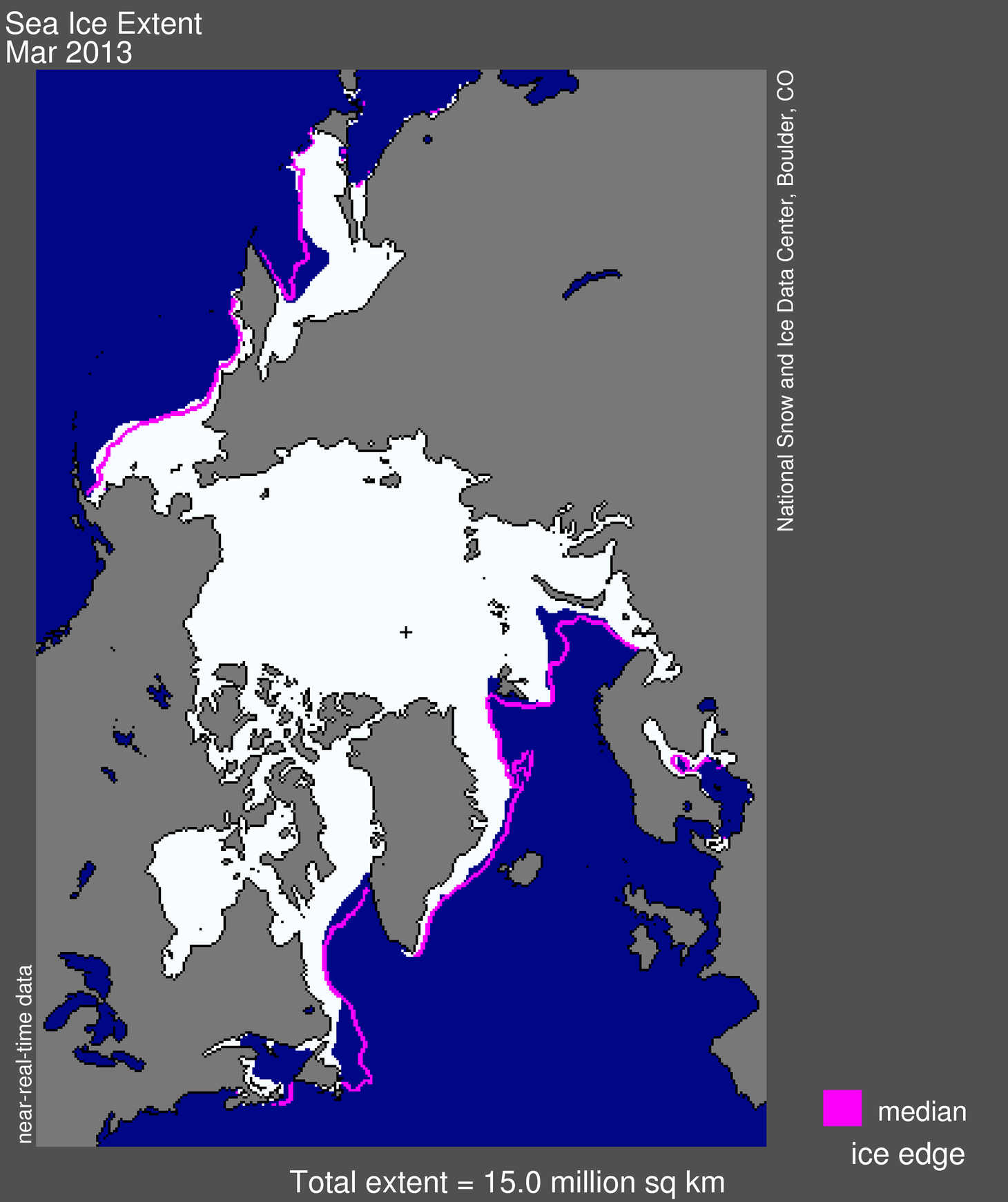
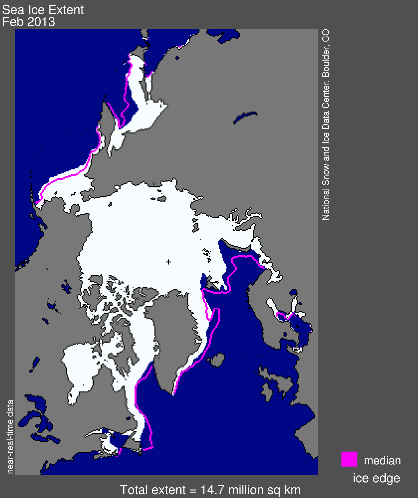
Figure 1. Arctic sea ice extent for August 18, 2013 was 5.94 million square kilometers (2.30 million square miles). The orange line shows the 1981 to 2010 median extent for that month. The black cross indicates the geographic North Pole. Sea Ice Index data. About the data

Credit: National Snow and Ice Data Center
High-resolution image

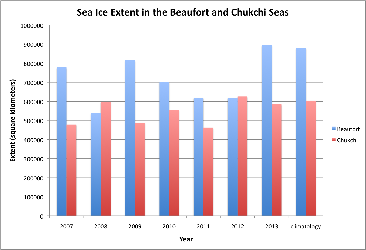
Sea ice retreat through the first half of August was near average, bringing the ice extent to 5.94 million square kilometers (2.30 million square miles). Sea ice extent continues to track well below average levels (average of 1981 to 2010), though remains within two standard deviations of the long-term mean. Retreat rates increased slightly in the western Beaufort Sea and Chukchi Sea, but ice cover remains extensive in those regions compared to 2012. Another major difference between ice extent during 2012 and this year is the much greater extent in the East Siberian Sea. Low ice extent in this region observed last year was in part attributed to the effects of the “Great Cyclone of 2012” (see previous post of August 14, 2012). On the eastern side of the Arctic near Europe and Greenland, the extent remains below average.

Conditions in context

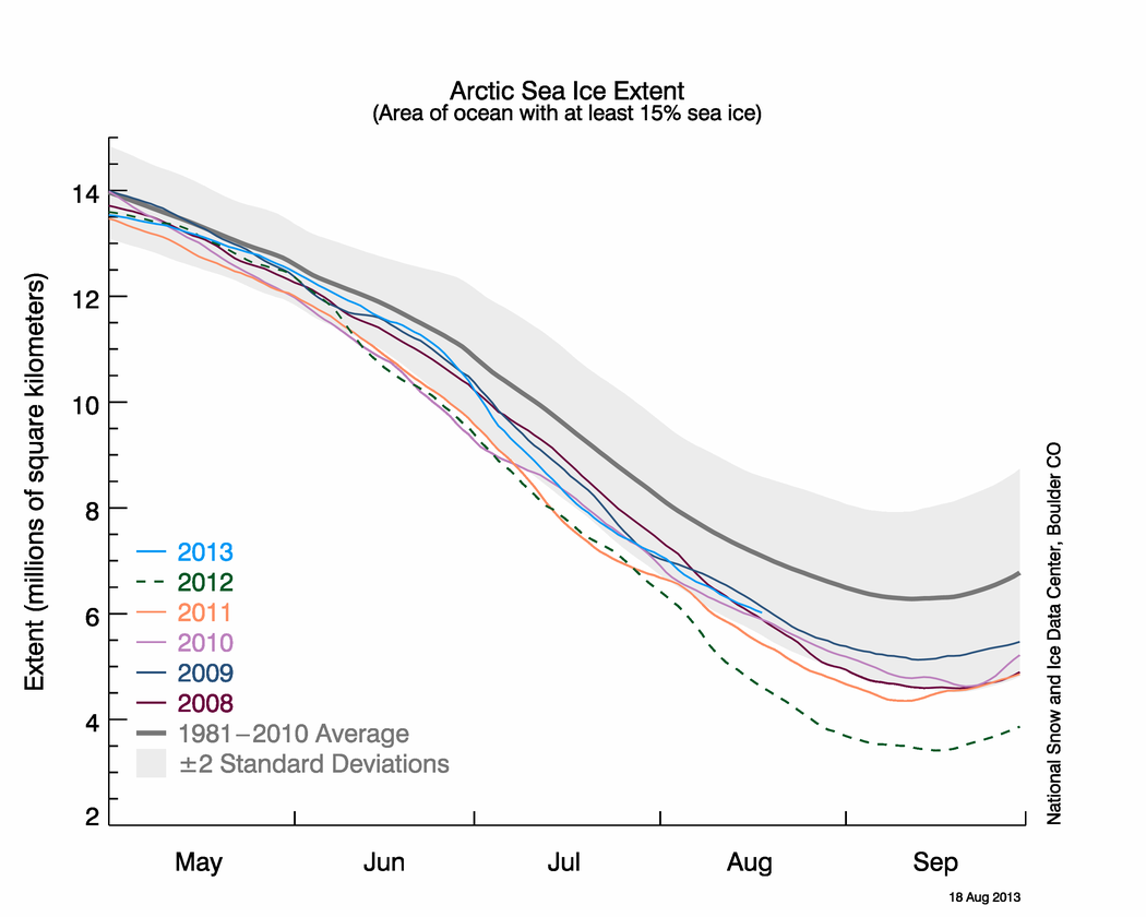
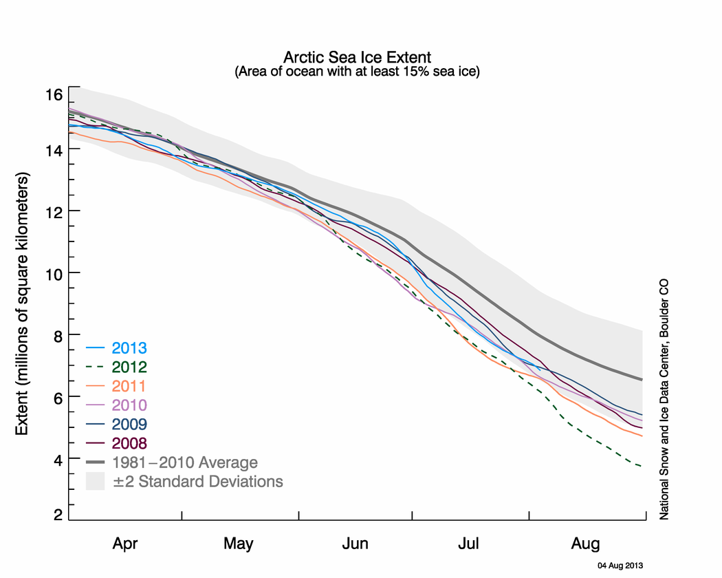
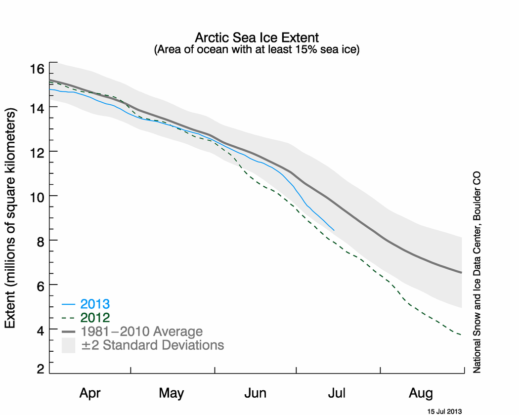
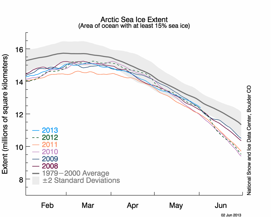
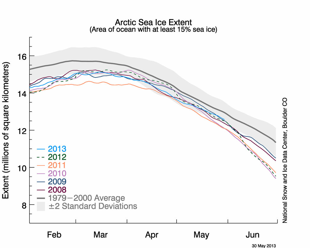
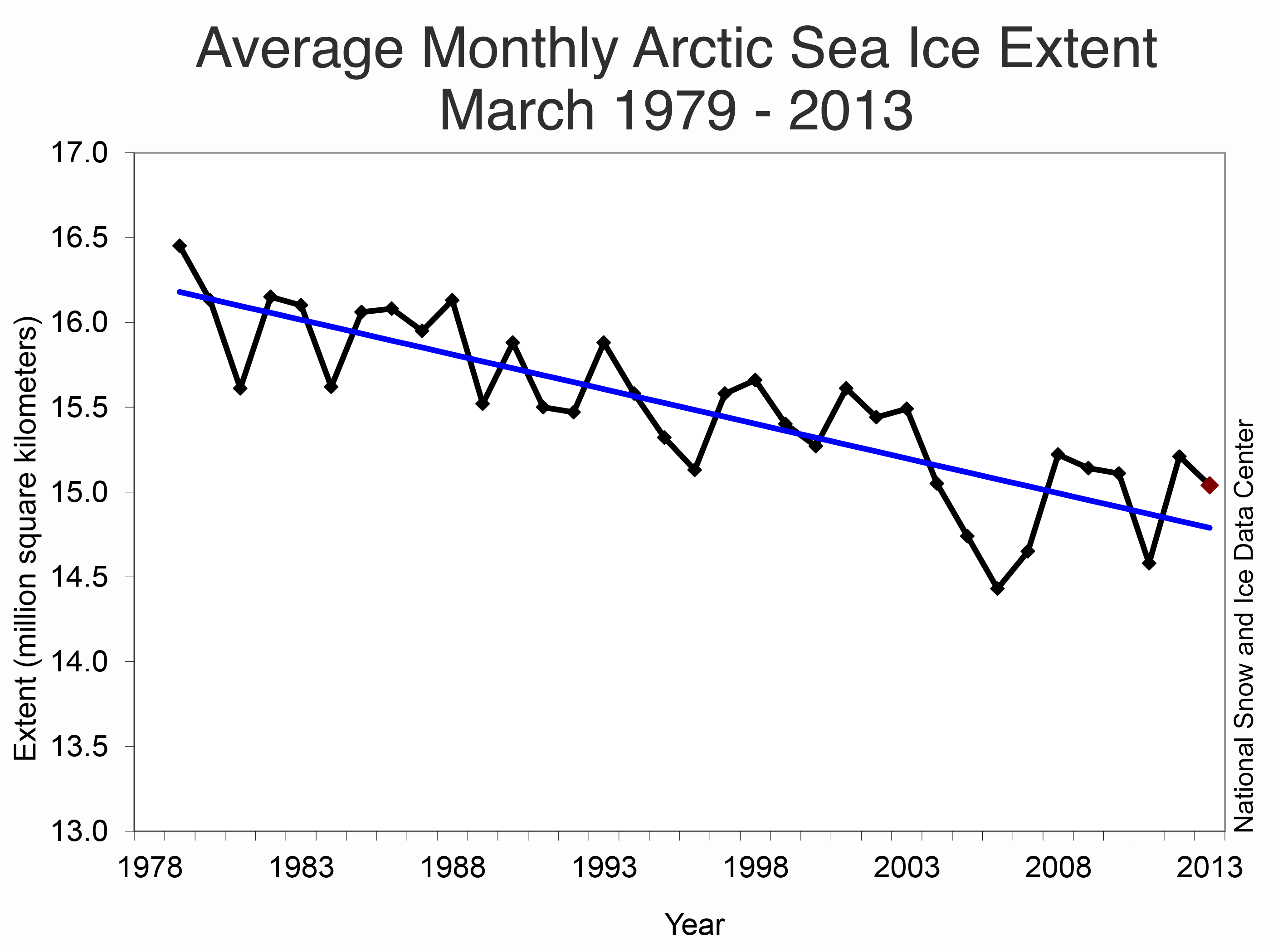
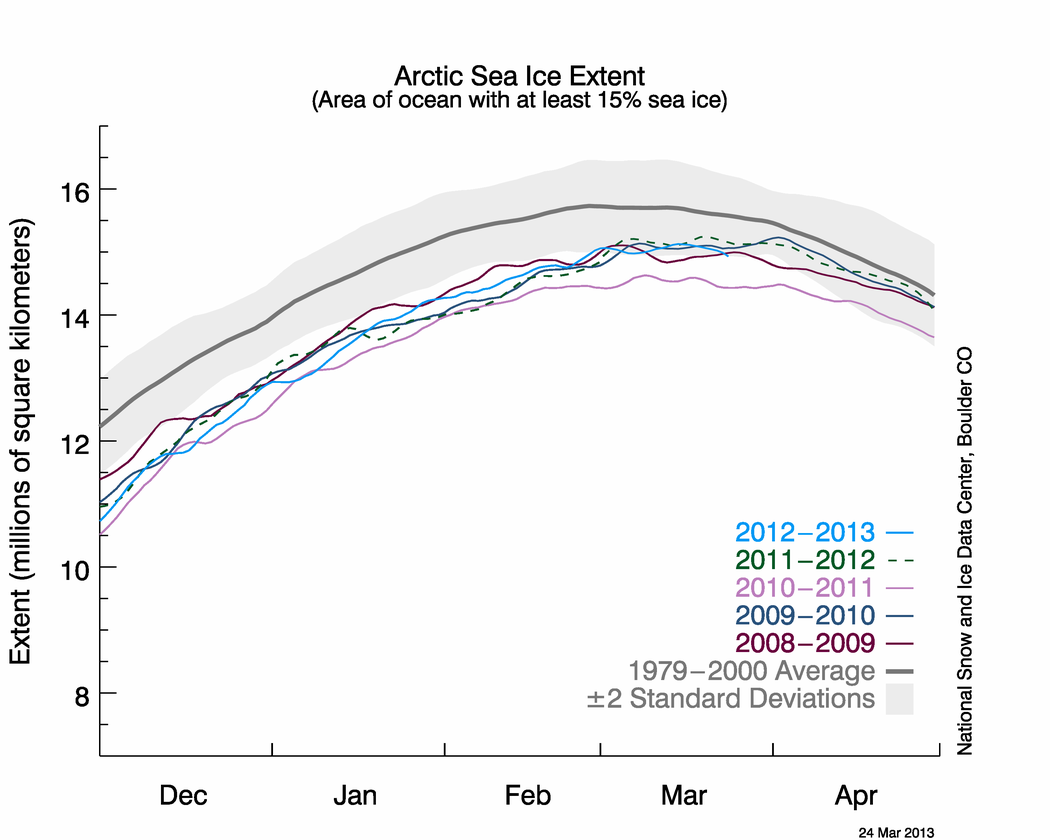
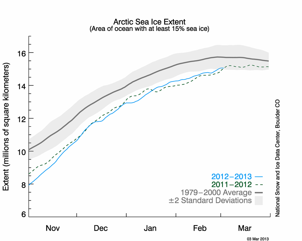
Figure 2. The graph above shows Arctic sea ice extent as of August 18, 2013, along with daily ice extent data for five previous years. 2013 is shown in blue, 2012 in green, 2011 in orange, 2010 in pink, 2009 in navy, and 2008 in purple. The 1981 to 2010 average is in dark gray. Sea Ice Index data.

Credit: National Snow and Ice Data Center
High-resolution image

The sea ice retreat rate averaged from August 1 to 18 was near average at approximately 75,000 square kilometers (29,000 square miles) per day. However, satellite data show extensive low-concentration areas within the ice cover, which appear to have developed in response to the frequent passage of storm systems. These weather patterns also result in lower-than-average air temperatures over the Arctic. Temperatures in the central Arctic at the 925 hPa level have been 2 to 4 degrees Celsius (4 to 7 degrees Fahrenheit) below average since late July.

A bit thin on top

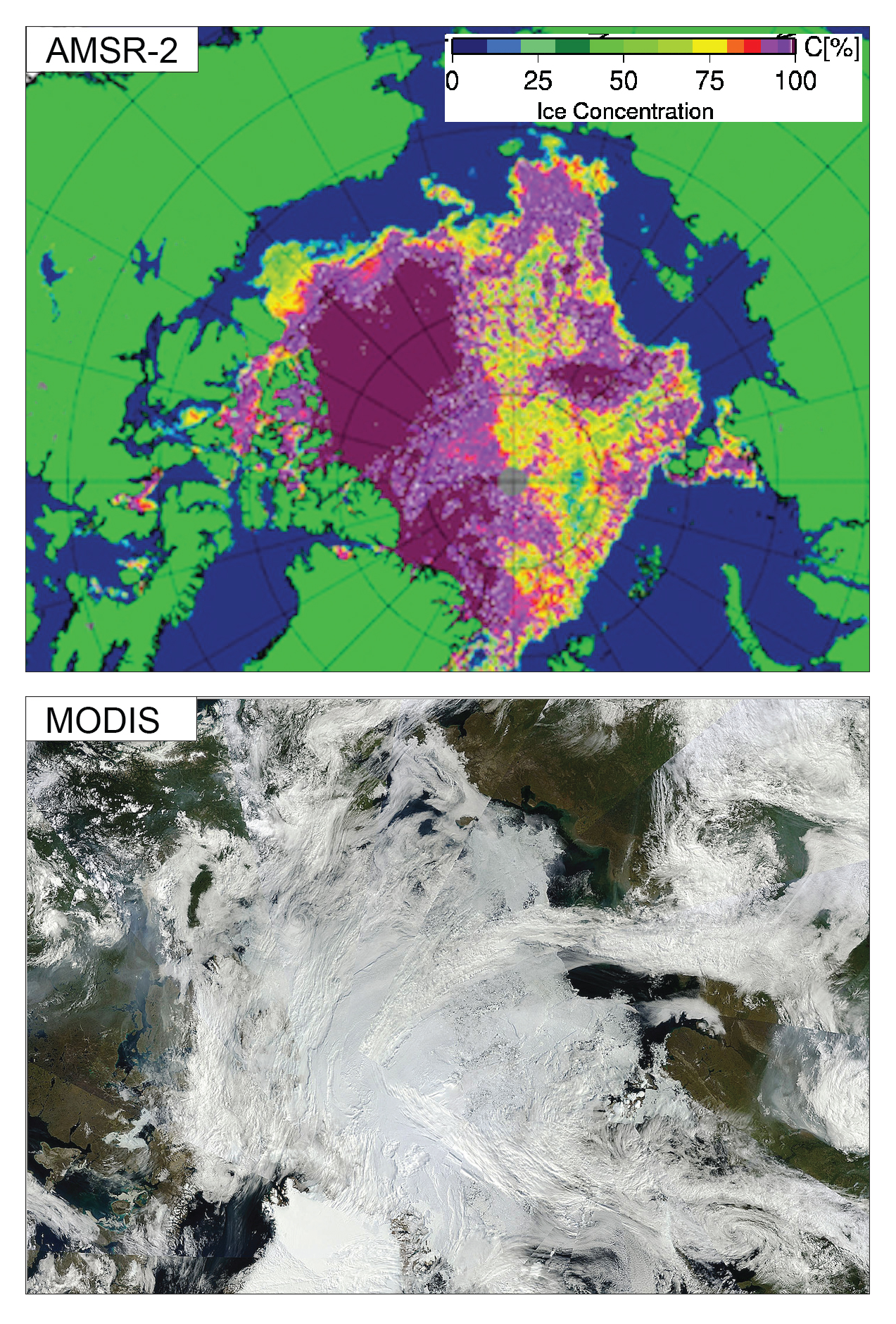
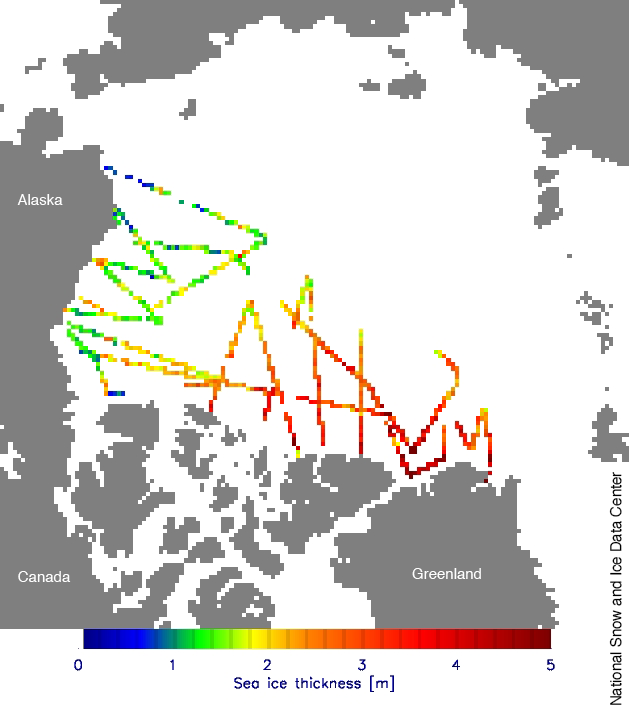
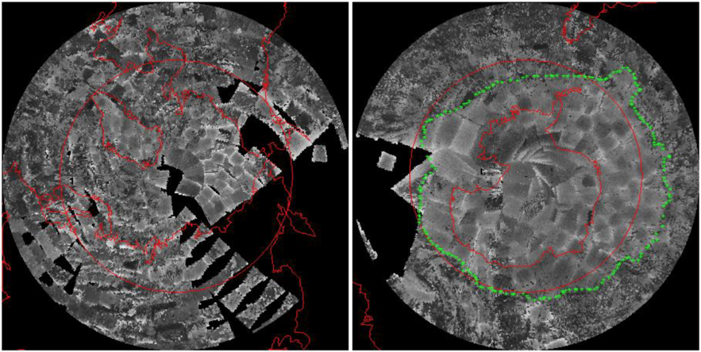
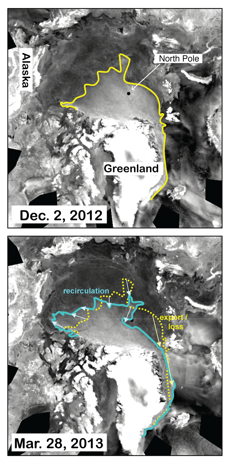
Figure 3. This composite shows an AMSR-2 sea ice concentration map (top) and a MODIS true-color composite image (bottom) of the Arctic for August 14, 2013. Clouds in the MODIS scene obscure some of the ice edges seen in the AMSR-2 data set.

Credit: University of Bremen/AMSR2; NASA/GSFC, Rapid Response
High-resolution image

Satellite data from the AMSR-2 instrument and MODIS show an unusually large expanse of low-concentration sea ice (20 to 80% cover) within our extent outline (15% or greater, using the SSM/I sensor) spanning much of the Russian side of the Arctic and extending to within a few degrees of the North Pole. A small area north of the Kara Sea has concentrations below 30%. This is likely in part a result of the dispersive effect of low-pressure systems that have migrated across the central Arctic over the past month. While some of the low concentrations recorded by AMSR-2 may be due to surface melt on sea ice, the MODIS image confirms that a large region is covered by isolated floes. The tendency towards a more open pack, with large areas of open water between ice floes, has increased in the past decade as the ice cover has thinned, as well as a tendency for formation of large polynyas (see ASINA posts for September 2006) and areas of pack detached from the main Arctic ice cover (such as mid-August 2012). The University of Washington’s Pan-Arctic Ice Ocean Modeling and Assimilation System (PIOMAS) model and other models of ice thickness continue to indicate thin ice cover this summer.

Not like last year

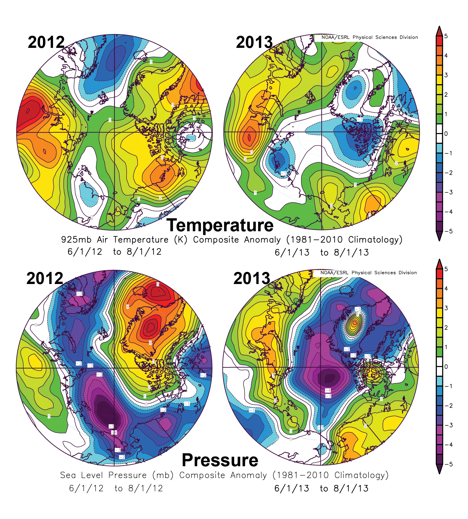
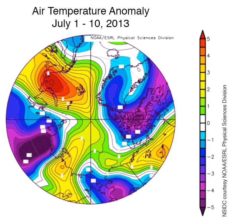
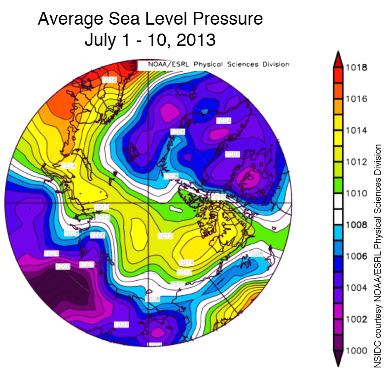
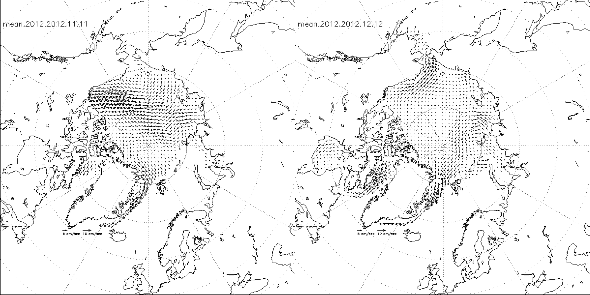
Figure 4. These images compare air temperatures at 925 mb (about 2500 feet above sea level) and air pressures at sea level for June through July, 2012, (left side) and June to July 2013 (right side).

Credit: NSIDC courtesy NOAA Earth System Research Laboratory Physical Sciences Division
High-resolution image

A comparison of average temperature and sea level pressure maps for June and July of 2012 (left diagrams) and 2013 (right diagrams) help us to understand why ice extent is higher in 2013. The pattern of unusually low pressure centered near the pole in 2013 has helped to spread the ice out and is consistent with generally cool conditions over much of the Arctic Ocean, inhibiting melt. By contrast, in the summer of 2012, a broad region of unusually high pressure centered over Greenland, in combination with below average pressure centered over the East Siberian and Chukchi seas, led to winds over the Beaufort Sea with a more southerly component than is usually the case, leading to warm conditions. That high pressure last year over Greenland also contributed to a record melt season for the Greenland ice sheet. Melt this year over the ice sheet has been more moderate, though still above rates seen in the 1990s. See our upcoming Greenland Today site post later this week.

Can’t get there from here

Figure 5. The graph above shows projections of ice extent from August 1 through September 30 based on observed retreat rates appended to the August 18, 2013 ice extent. None of the observed patterns of the past few years, or the mean loss rates, bring the ice extent below 4.0 million square kilometers (1.56 million square miles). Sea Ice Index data.

Credit: National Snow and Ice Data Center
High-resolution image

Projections of the likely minimum extent this year based on retreat rates from past years argue that it is highly unlikely that sea ice will surpass the record-setting low extent seen in 2012. With retreat rates similar to those of 2007 to 2012, the minimum extent would be near 5.0 million square kilometers (2.0 million square miles) in mid-September.

Record extent in the Antarctic

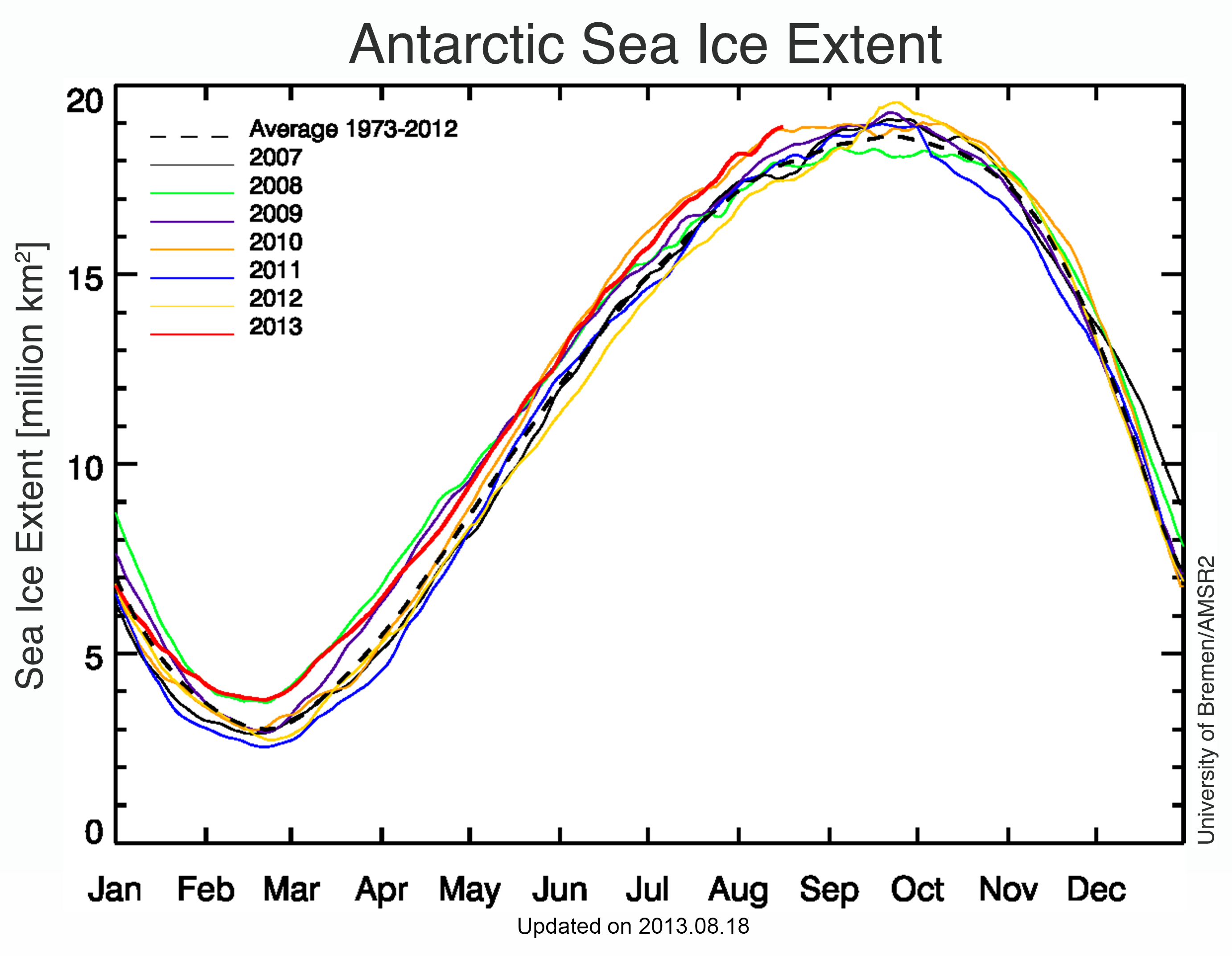
Figure 6. Antarctic daily sea ice extents for 2013, 2010, 2007, and the 1981 to 2010 mean for the past few months. Sea Ice Index data.

Credit: University of Bremen/AMSR2
High-resolution image

Antarctic sea ice extent for August 19 is 18.70 million square kilometers (7.22 million square miles), a record or near-record high level (August 19, 2010 was similarly high), led by unusually extensive ice in the Bellingshausen, Amundsen, and Ross seas, and in the western Indian Ocean sector. Climate conditions since June have been variable, but the most recent surge in ice growth has occurred during a period of unusually high pressure over the center of the continent, resulting in a slowing of the circumpolar winds, warm winter conditions for the central ice sheet areas (Vostok Station and Amundsen-Scott South Pole Station both had periods of spring-like -30s earlier in the month), and cold conditions in the Bellingshausen, allowing ice to grow extensively there.

Following rapid ice loss in the first half of July, the pace of seasonal ice retreat slowed the rest of the month partly due to the return of a stormy weather pattern over the central Arctic Ocean. The timing of melt onset for 2013 was in general unremarkable. Ice extent remains below average on the Atlantic side of the Arctic, and near average in the Beaufort and Chukchi seas, and along the Eurasian coast.

Overview of conditions

Figure 1. Arctic sea ice extent for July 2013 was 8.45 million square kilometers (3.26 million square miles). The magenta line shows the 1981 to 2010 median extent for that month. The black cross indicates the geographic North Pole. Sea Ice Index data. About the data

Credit: National Snow and Ice Data Center
High-resolution image

Sea ice extent for July 2013 averaged 8.45 million square kilometers (3.26 million square miles). This is 1.25 million square kilometers (483,000 square miles) below the 1981 to 2010 average for the month (Note that on July 2, 2013, NSIDC began using a new 30-year baseline for analyzing sea ice.). Ice extent remains below average on the Atlantic side of the Arctic, and is near average to locally above average in the Beaufort and Chukchi seas and along much of the Eurasian coast.

Conditions in context

Figure 2. The graph above shows Arctic sea ice extent as of August 4, 2013, along with daily ice extent data for five previous years. 2013 is shown in blue, 2012 in green, 2011 in orange, 2010 in pink, 2009 in navy, and 2008 in purple. The 1981 to 2010 average is in dark gray. Sea Ice Index data.

Credit: National Snow and Ice Data Center
High-resolution image

While sea ice extent retreated rapidly through the first two weeks of July when the weather was dominated by high pressure and clockwise winds over the central Arctic Ocean, the pace of ice loss for the last half of the month was slower. This was partly due to the return of a stormy pattern that brought more counterclockwise winds and cool conditions, and spread the ice out. This spreading of the ice, or ice divergence, can result in more dark open water areas between individual floes that enhance absorption of the sun’s energy, leading to more lateral and basal melting. However, the effects of cooler conditions and ice divergence on the overall ice extent depend in part on the thickness of the ice. Historically, stormy summers tended to end up with more ice than summers characterized by high pressure and few storms. As the ice cover has thinned, stormy conditions may actually help to remove more ice.

July 2013 compared to previous years

Figure 3. Monthly July ice extent for 1979 to 2013 shows a decline of 7.4% per decade relative to the 1981 to 2010 average.

Credit: National Snow and Ice Data Center
High-resolution image

Overall, extent dropped an average of 105,000 square kilometers (41,000 square miles) per day through the month, the second fastest July ice loss in the satellite record after 2007, and much higher than the 1981 to 2010 average. However, this number averages the rapid ice loss during the first half of the month with the slower loss during the second half of the month. July 2013 was the fifth lowest July in the 1979 to 2013 satellite record, and 540,000 square kilometers (208,000 square miles) above the record low in 2011. The monthly trend is ‑7.4% per decade relative to the 1981 to 2010 average (also ‑7.1% per decade relative to the old 1979 to 2000 baseline).

Summer storms

Summer is the stormiest season over the central Arctic Ocean, but the situation can vary greatly within a month (as has been the case for July 2013), from month to month, and year to year. The summer storms in this region can occasionally be quite strong and there has been some discussion that, like hurricanes, strong Arctic storms should be named, perhaps drawing on the Inuit language. Last August, a cyclone in the region attained a central pressure as low as 964 hPa, with attendant strong winds. As just discussed, summers characterized by stormy conditions tend to end up with more sea ice than summers characterized by high pressure. However, the effects of an individual strong storm can be complex. It appears that the August 2012 storm was attended by a modest acceleration in the pace of summer ice loss. While the middle of July 2013 also saw a storm over the central Arctic Ocean with a central pressure of 977 hPa, this year’s event has not led to a strong ice loss.

A note on melt ponds

Figure 4. These comparison images show the North Pole Web Cam on July 25, 2013 (top), and July 30, 2013 (bottom).

Credit: North Pole Environmental Observatory
High-resolution image

There have been confusion and misinformation on several Arctic- and climate-focused Web blogs regarding the presence of a lake at the North Pole, as viewed from the North Pole Webcam, which is part of the North Pole Environmental Observatory (NPEO). First, the webcam is not at the North Pole. Because of the drift of the ice, as of this week it is actually located at about 84 degrees North near the prime meridian. Second, the so-called lake is nothing more than a large summer melt pond atop the ice cover, and is not, as some have said, a hole or a polynya in the ice cover. While quite extensive by July 26, the pond appears to have largely disappeared by July 30, by draining off the sea perhaps through a fracture, followed by a dusting of snow. See the NPEO’s FAQ on the melt ponding this year.

*Note: A reader called our attention to details in the North Pole Web Cam images of the recent melt pond. After examining these and conferring with other researchers, we have revised the sentence that reads: “While quite extensive by July 26, the pond appears to have largely disappeared by July 30 under what is probably a thin layer of ice covered with a dusting of snow.” The updated version now reads “While quite extensive by July 26, the pond appears to have largely disappeared by July 30, by draining off the sea perhaps through a fracture, followed by a dusting of snow.”

 Onset of summer melt

Figure 5. The graph above compares melt onset dates for sectors of the Arctic Ocean.

Credit: National Snow and Ice Data Center
High-resolution image

The same satellite passive microwave data that NSIDC uses to determine sea ice extent can also be used to determine the date of the onset of summer melt over the sea ice cover. Compared to the average over the period 1981 to 2010, the date of melt onset, as assessed for different sectors of the Arctic Ocean, was largely unremarkable. It was slightly earlier than average in some sectors but later than average in others.

Further reading

Serreze, M. C. and A. P. Barrett. 2008. The summer cyclone maximum over the central Arctic Ocean. Journal of Climate 21, doi:10.1175/2007JCLI1810.1.

Kwok, R. and N. Untersteiner. 2011. The thinning of the Arctic sea ice. Physics Today 64(4), April 2011, doi:10.1063/1.3580491.

Rosel, A., L. Kaleschke, and G. Birnbaum. 2011. Melt ponds on Arctic sea ice determined from MODIS satellite data using an artificial neural network. The Cryosphere Discussions 5, 2991–3024, doi:10.5194/tcd-5-2991-2011.

Sea ice extent retreated fairly rapidly through the first two weeks of July as a high pressure cell moved into the central Arctic, bringing warmer temperatures over much of the Arctic Ocean. Ice extent remains below average on the Atlantic side of the Arctic, and is near average to locally above average in the Beaufort and Chukchi seas and along much of the Eurasian coast.

Overview of conditions

Figure 1. Arctic sea ice extent for July 15, 2013 was 8.20 million square kilometers (3.17 million square miles). The orange line shows the 1981 to 2010 median extent for that month. The black cross indicates the geographic North Pole. Sea Ice Index data. About the data

Credit: National Snow and Ice Data Center
High-resolution image

While the rate of Arctic sea ice loss is normally fastest during July, the warmest month of the year, ice loss was even faster than usual over the first two weeks of July 2013. As a result, on July 15 extent came within 540,000 square kilometers (208,000 square miles) of that seen in 2012 on the same date. The ice loss is dominated by retreat on the Atlantic side of the Arctic, including the East Greenland, Kara and Laptev seas, and Baffin Bay. In the Beaufort and Chukchi seas and much of the Eurasian coast, the ice cover remains fairly extensive, especially compared to recent summers. Compared to the 1981 to 2010 average, ice extent on July 15, 2013 was 1.06 million square kilometers (409,000 square miles) below average.

Conditions in context

Figure 2. The graph above shows Arctic sea ice extent as of July 15, 2013, along with daily ice extent data for 2012, the record low year. 2013 is shown in blue, and 2012 in green. The gray area around the average line shows the two standard deviation range of the data. Sea Ice Index data.

Credit: National Snow and Ice Data Center
High-resolution image

During the first two weeks of July, ice extent declined at a rate of 132,000 square kilometers (51,000 square miles) per day. This was 61% faster than the average rate of decline over the period 1981 to 2010 of 82,000 square kilometers (32,000 square miles) per day. The fast pace of ice loss was dominated by retreat in the Kara and East Greenland seas, where the ice loss rate from July 1 to 12 was -16,409 and -17,678 square kilometers (-6,336 and -6,826 square miles) per day, respectively. The Laptev Sea ice retreated at about half that rate, at -8,810 square kilometers (-3,402 square miles) per day.  In contrast, on the Pacific side, sea ice has been slow to retreat. During the first part of July, the rate of ice loss in the Beaufort and Chukchi seas was only -3,375 and -6,829 square kilometers (-1,303 and -2,637 square miles), respectively.

A change in the weather

Figure 3a. This image of air temperature anomalies at the 925 hPa level from July 1 to 10 July 10, 2013 shows higher than average temperatures over the Arctic, especially over the Kara Sea. Air temperature anomalies are relative to the 1981 to 2010 average.

Credit: NSIDC courtesy NOAA Earth System Research Laboratory Physical Sciences Division
High-resolution image

Figure 3b. This image of average sea level pressure from July 1 to 10, 2013 shows high pressure in the central Arctic.

Credit: NSIDC courtesy NOAA Earth System Research Laboratory Physical Sciences Division
High-resolution image

Temperatures at the 925 hPa level for the first two weeks in July were 1 to 3 degrees Celsius (2 to 5 degrees Fahrenheit) above average over much of the Arctic Ocean and as much as 5 degrees Celsius (9 degrees Fahrenheit) above average over the Kara Sea, where ice loss was pronounced. In contrast, temperatures over Alaska, Siberia and the Canadian Arctic were 3 to 5 degrees Celsius (5 to 9 degrees Fahrenheit) lower than average.

Warmer conditions have been paired with a shift in the atmospheric circulation, with a high pressure cell at sea level pressure moving into the central Arctic, replacing then pattern of low pressure that dominated the month of June. This has helped to bring in warm air from the south over the Arctic Ocean. This pattern has also helped to create open water areas in the Laptev Sea because offshore winds push the ice away from shore.

Slow ice retreat along coastal Alaska and Canada

Figure 4. This graph of sea ice extent in the Beaufort and Chukchi Seas as of July 12 each year shows an increase in ice extent in the Beaufort Sea over the last seven summers.

Credit: NSIDC
High-resolution image

The slow retreat of sea ice in the Beaufort Sea has resulted in the most extensive ice cover seen there in the last seven summers (Figure 4). Ice extent also remains rather extensive in the Chukchi Sea, though other recent years have seen more ice at this same time of year, particularly in 2012, when Shell was forced to delay drilling operations and reduce the number of wells planned. Despite extensive ice cover, visible imagery from the Moderate Resolution Imaging Spectroradiometer (MODIS) satellite instrument shows melt is well underway.

Arctic sea ice continues to track below average but remains well above the levels seen last year. The relatively slow ice loss is a reflection of the prevailing temperature and wind patterns. As of July 1, NSIDC Arctic Sea Ice News and Analysis and the Sea Ice Index have transitioned to a new 30-year baseline period, 1981 to 2010.

Overview of conditions

Figure 1. Arctic sea ice extent for June 2013 was 11.58 million square kilometers (4.47 million square miles). The magenta line shows the 1981 to 2010 median extent for that month. The black cross indicates the geographic North Pole. Sea Ice Index data. About the data

Credit: National Snow and Ice Data Center
High-resolution image

June is a transition period for Arctic sea ice as 24-hour daylight reigns, and melt reaches towards the North Pole. Thus it is an appropriate time for NSIDC to transition to a new 30-year baseline period, also called a “climate normal.” The satellite record is now long enough to allow NSIDC to match current National Ocean and Atmospheric Administration (NOAA) and World Meteorological Organization (WMO) standard baselines of 1981 to 2010 for weather and climate data. Full details of the changes and the implications for NSIDC sea ice statistics are described in the NSIDC Sea Ice Index.

Average sea ice extent for June 2013 was 11.58 million square kilometers (4.47 million square miles). This was 310,000 square kilometers (120,000 square miles) below the 1981 to 2010 average (the new baseline period) of 11.89 million square kilometers (4.59 million square miles). In comparison, the 1979 to 2000 period that we previously used averaged 12.16 million square kilometers (4.70 million square miles). June 2013 was 760,000 square kilometers (293,000 square miles) above the record low June extent in 2010.

Conditions in context

Figure 2a. The graph above shows Arctic sea ice extent as of June 30, 2013, along with daily ice extent data for five previous years. 2013 is shown in blue, 2012 in green, 2011 in orange, 2010 in pink, 2009 in navy, and 2008 in purple. The 1981 to 2010 average is in dark gray. Sea Ice Index data.

Credit: National Snow and Ice Data Center
High-resolution image

Figure 2b. The graph above shows Arctic sea ice extent as of June 30, 2013, along with daily ice extent data for 2012, the record low year, and both the new and old baseline average periods. The 1981 to 2010 average is shown by a dark gray line. The gray area around this average line shows the two standard deviation range of the 1981 to 2010 average. The 1979 to 2000 average is shown by a blue line. The light purple shading around this line shows the two standard deviation range of the 1979 to 2000 average.

Credit: National Snow and Ice Data Center
High-resolution image

Although the rate of ice loss increased toward the end of June, overall ice has retreated more slowly this summer compared to last summer, reflecting patterns of atmospheric circulation and air temperature. Average June temperatures at the 925 mb level were average to slightly below average over most of the Arctic Ocean, contrasting with above average temperatures over most of the surrounding land. This temperature pattern is associated with unusually low sea level pressure centered near the North Pole. This type of circulation pattern is known to slow the summer retreat of ice, not just because it fosters cool conditions, but also because the pattern of cyclonic (counterclockwise) winds tends to spread the ice out. An interesting regional aspect of this pattern is that on the heels of unusually cold spring conditions, the Alaska interior experienced some days of record high temperatures during June.

June 2013 compared to previous years

Figure 3. Monthly June ice extent for 1979 to 2013 shows a decline of 3.6% per decade relative to the 1981 to 2010 average.

Credit: National Snow and Ice Data Center
High-resolution image

Sea ice extent declined steadily through most of the month, in sharp contrast to last year when June experienced a record fast pace of sea ice retreat. There was a speed-up in ice loss toward the end of the month. Overall, extent dropped an average of 70,300 square kilometers (27,000 square miles) per day through the month, slightly higher than the 1981 to 2010 average.

June 2013 was the 11th lowest June in the 1979 to 2013 satellite record, 760,000 square kilometers (293,000 square miles) above the record low in 2010. The monthly trend is -3.6% percent per decade relative to the 1981 to 2010 average (also -3.6% per decade relative to the old 1979 to 2000 baseline).

An Arctic pre-conditioned for rapid summer ice loss?

Figure 4. Data from NASA Operation IceBridge flights over the Arctic Ocean during March and April 2013 indicate thick ice along the Greenland coast (shown in reds), but thin ice north of Alaska (blues and greens).

Credit: National Snow and Ice Data Center/NASA Operation IceBridge
High-resolution image

Through most of June, we did not see the precipitous decline in ice extent that was observed in June 2012 and 2007 (the years with the lowest and second lowest September ice extent in the satellite record). However, the rate of ice loss did increase in late June. Ice cover this spring was very thin in parts of the Arctic, suggesting that large areas may soon start melting out completely. Much depends on whether the atmospheric circulation pattern seen in June persists through July.

NASA Operation IceBridge data collected during March and April indicated thick ice along the Greenland coast (5 meters, or 16 feet or more), but thin ice north of Alaska in the Beaufort and Chukchi seas, ranging from 1 to 1.5 meters (3 to 5 feet) in most areas and as low as 0.5 meters (approximately 2 feet) in others. These thin areas are quite likely refrozen leads, linked to the major fracturing events that occurred in the region during February and March. According to Andrew Shepherd at the University of Leeds, preliminary results from the European Space Agency CryoSat satellite suggest that the ice pack was 8% thinner in March 2013 compared to March 2012.

An ocean of small floes

Figure 5. High-resolution passive microwave data from AMSR2 on June 26, 2013 (left image) shows areas of low ice concentration near the North Pole, indicated in greens. Visible imagery from MODIS on June 27, 2013 (right image) of the inset area reveals a fractured ice surface with small floes.

Credit: University of Bremen/AMSR2; NASA/GSFC, Rapid Response
High-resolution image

High-resolution passive microwave concentration data from the Japan Aerospace Exploration Agency AMSR2 sensor, produced by the University of Bremen, indicate a highly unusual region of broken-up ice near the North Pole. Development of this low concentration ice may have been assisted by the cyclonic atmospheric pattern noted earlier.

While the AMSR2 image in Figure 5 suggests concentrations as low as 50%, visible imagery from the MODIS sensor on the NASA Aqua satellite indicate that AMSR2 is underestimating concentration, likely due to biases from surface melt.

Still, the MODIS data do confirm that the ice is highly fractured with numerous small floes. Such small floes are more easily melted from the sides and the bottom by ocean waters that are exposed to the 24-hour sunlight. It remains to be seen how many of these small floes will ultimately melt completely.

This July, NSIDC plans to change the baseline climatological period for Arctic Sea Ice News and Analysis and the Sea Ice Index, the data set we use for our sea ice analysis. We are making this change to match the comparison time frames used by other climate research.

Until now, we have used the 22-year period 1979 to 2000 when comparing current sea ice extent to past conditions. When NSIDC first began to monitor and analyze sea ice extent, a longer period was not available. Since the satellite record is now extended, we are choosing to move to a more standard 30-year reference period, from 1981 to 2010.

A 30-year period typically defines a climatology (comparsion period) and is the standard used by organizations such as the World Meteorological Organization (WMO) and the U.S. National Oceanic and Atmospheric Administration (NOAA). Thirty years is considered long enough to average out most variability from year to year, but short enough so that longer-term climate trends are not obscured.

These maxims about climate averages come from the world of weather and climate. Sea ice responds to changes in energy or heat differently from other systems on Earth. So the assumptions behind the use of 30-year averages for weather may not hold true for sea ice, particularly in light of the rapid decrease and repeated record low minimum extents in the Arctic during the past decade. However, matching the 1981 to 2010 period brings us in line with other climate research.

The monthly and daily sea ice extent images and data values will not change, but data and images that are based on the average or median will change. For example, the trend plot for sea ice extent will have a different scale, and the value of the slope, expressed as change in percent per decade, will change, because this value is relative to the average period. On the the monthly and daily extent images, the position of the average extent lines will change.

In our July analysis, we will provide more information to help readers put these changes into the larger context of changing climate and changing ice.

Arctic sea ice extent declined at a near-average rate through May, but overall it remained below average compared to the 1979 to 2000 average. The Arctic Oscillation (AO) varied through the month between modest positive and negative phases. Winds from the north and northwest and persistent snow cover over central Alaska made much of the month unusually cold there. The last part of the month saw much higher temperatures.

Overview of conditions

Figure 1. Arctic sea ice extent for May 2013 was 13.10 million square kilometers (5.06 million square miles). The magenta line shows the 1979 to 2000 median extent for that month. The black cross indicates the geographic North Pole. Sea Ice Index data. About the data

Credit: National Snow and Ice Data Center
High-resolution image

Sea ice extent in May 2013 averaged 13.10 million square kilometers (5.06 million square miles). This is 500,000 square kilometers (193,000 square miles) below the 1979 to 2000 average for the month. As has been the case for the past several years, ice extent was below average in the Barents Sea on the Atlantic side of the Arctic. Greater than average ice extent prevailed on the Pacific side of the Arctic in the Bering Sea and Sea of Okhotsk.

Conditions in context

Figure 2. The graph above shows Arctic sea ice extent as of June 2, 2013, along with daily ice extent data for five previous years. 2013 is shown in blue, 2012 in green, 2011 in orange, 2010 in pink, 2009 in navy, and 2008 in purple. The 1979 to 2000 average is in dark gray. The gray area around this average line shows the two standard deviation range of the data. Note: 2011 was inadvertently omitted from this graph; corrected June 17. Sea Ice Index data.

Credit: National Snow and Ice Data. High resolution image

The AO varied through the month between modest positive and negative phases. However, May was characterized by a broad region of unusually low pressure covering much of the western Arctic, namely the Beaufort, Chukchi, and East Siberian seas. Earlier large-scale fracturing of the sea ice off the northeast coast of Alaska and north of the Canadian Archipelago mentioned in our past post was linked to a pattern of high pressure over the Arctic and a strongly negative phase of the AO.

There are several open water areas, or polynyas, along the Arctic coast, as is typical for this time of year. Small patches of open water are present along the Laptev Sea coast north of Russia, and at the northern end of Baffin Bay. These will expand as summer melting and warmer conditions progress in the Arctic.

May 2013 compared to previous years

Figure 3. Monthly May ice extent for 1979 to 2013 shows a decline of -2.24 percent per decade.

Credit: National Snow and Ice Data Center
High-resolution image

May 2013 was the tenth lowest May in the satellite record, 390,000 square kilometers (151,000 square miles) above the record low of 12.58 million square kilometers (4.86 million square kilometers) in 2004.*

Through the month of May this year, extent declined at an average rate of 36,400 square kilometers (14,100 square miles) per day, slower than the 1979 to 2000 average of 44,100 square kilometers (17,000 square miles) per day.

*Note: We originally stated that the record low had occurred in May 2011. After reviewing the data, we corrected this statement. See the Sea Ice Index for data on past May ice extent.

Snow cover update

Figure 4. This snow cover anomaly map shows the difference between snow cover for May 2013, compared with average snow cover for May from 1971 to 2000. Areas in orange and red indicate lower than usual snow cover, while regions in blue had more snow than normal.

Credit: National Snow and Ice Data Center, courtesy Rutgers University Global Snow Lab
High-resolution image

Monthly snow cover anomaly data from the Rutgers University Global Snow Lab  show that snow cover for the month of May was significantly low in eastern Siberia, northern Europe, and the Rocky Mountains in North America. Data also show a few greater-than-average regions in Alaska—contributing to the lower temperatures there—and on  the Tibetan Plateau.

Weekly and daily data from the Global Snow Lab show that May began with greater-than-average snow cover in Tibet and the Great Plains of Canada and the United States. By the end of the month, however, snow extent was near average to lower than average throughout the Northern Hemisphere, and much lower than average in northeastern Siberia. Overall, snow cover in May 2013 was the lowest on record in forty-seven years of data for Eurasia, and third lowest overall for the Northern Hemisphere, trailing only 2012 and 2010.

Chilly in Alaska

Figure 5. This image shows air temperature anomalies at the 925 hPa level averaged for May 2013, compared to averages over the period 1981 to 2010. Temperatures were lower than average over Alaska, while temperatures across much of Siberia were above average.

Credit: NSIDC courtesy NOAA Earth System Research Laboratory Physical Sciences Division
High-resolution image

Lower than average temperatures were the rule this past month for both Greenland and Alaska, while temperatures across much of Siberia were above average. Temperatures over central Alaska at the 925 hPa level were 4 to 5 degrees Celsius (7 to 9 degrees Fahrenheit) colder than usual, making this one of the coldest springs on record for cities like Fairbanks. These low temperatures can be linked to winds from the north and northwest over central Alaska and persistent snow cover. However, the end of the month saw much higher temperatures, reaching more than 80 degrees Fahrenheit (27 degrees Celsius) in Fairbanks.

Because of the low temperatures, ice on the Tanana River, which runs through Fairbanks, Alaska, broke up on May 20 at 2:41 p.m.—the latest date and time on a record which extends for nearly a century. Ice break-up has been carefully recorded at the town of Nenana, about 70 kilometers (44 miles) downstream on the Tanana River from Fairbanks, by timing the tipping of a large tripod erected on the river ice. This is a matter of some importance for Alaskans, as there is a large statewide lottery based on picking the exact time of ice break-up. In most years, winning this lottery requires picking the time to the precise minute of tipping. Congratulations to Warren and Yvonne Snow, for your excellent climate forecasting (and on having a wonderful last name)!

Arctic sea ice extent declined at an approximately average rate through April. While the Arctic Oscillation was in its negative phase for most of winter, in mid April it turned positive. This helped to bring in warm air over Eurasia, although air temperatures over the sea ice cover remain below freezing.

Overview of conditions

Figure 1. Arctic sea ice extent for April 2013 was 14.37 million square kilometers (5.54 million square miles). The magenta line shows the 1979 to 2000 median extent for that month. The black cross indicates the geographic North Pole. Sea Ice Index data. About the data

Credit: National Snow and Ice Data Center
High-resolution image

Sea ice extent averaged for the month of April 2013 was 14.37 million square kilometers (5.54 million square miles). This is 630,000 square kilometers (243,000 square miles) below the 1979 to 2000 average for the month, and is the seventh-lowest April extent in the satellite record.

In the earlier part of the satellite data record, average April extent remained above 15 million square kilometers (5.8 million square miles). Since 1989 the extent has mostly remained between 14 and 15 million square kilometers (5.4 and 5.8 million square miles). The years 1993 and 1999 were exceptions, when extent exceeded 15 million square kilometers (5.8 million square miles), as well as 2006 and 2007, when extent dropped below 14 million square kilometers (5.4 million square miles).

A large area of open water has started to form around Franz Josef Land and north of Svalbard. Polynyas are also appearing in the Kara and East Siberian seas.

The walrus and whaling season has begun in Arctic Alaska. The Study of Environmental Arctic Change (SEARCH) Sea Ice for Walrus Outlook (SIWO) is now providing weekly sea ice outlooks as a resource for Alaska Native subsistence hunters, coastal communities, and others interested in sea ice and walrus or whales. With spring sea ice conditions being thinner and less predictable than in the past due to warming in the Arctic, the sea ice outlook helps hunters plan their activities.

Conditions in context

Figure 2. The graph above shows Arctic sea ice extent as of April 30, 2013, along with daily ice extent data for five previous years. 2013 is shown in blue, 2012 in green, 2011 in orange, 2010 in pink, 2009 in navy, and 2008 in purple. The 1979 to 2000 average is in dark gray. The gray area around the average line shows the two standard deviation range of the data. Note: 2011 was inadvertently omitted from this graph; corrected June 17. Sea Ice Index data.

Credit: National Snow and Ice Data Center
High-resolution image

Through the month of April, the Arctic lost 1.5 million square kilometers of ice (444,000 square miles), which is slightly higher than the average for the month. Air temperatures at the 925 hPa level (approximately 3,000 feet above sea level) in April were 5 to 7 degrees Celsius (9 to 13 degrees Fahrenheit) higher than average in the East Siberian Sea and 3 to 5 degrees Celsius (5 to 9 degress Fahrenheit) higher than average in the Kara Sea. Temperatures were 3 to 5 degrees Celsius (5 to 9 degrees Fahrenheit) below average over Alaska. The dominant feature of the Arctic sea level pressure field for April 2013 was unusually high pressure over Alaska and Siberia and below average pressure over the Kara and Barents seas.  During the middle of the month, the Arctic Oscillation switched from a negative to a positive phase, with anomalously high sea level pressure over Alaska combined with below average pressure over Greenland and the North Atlantic. This brought in warm air over Eurasia, and above average air temperatures throughout the eastern Arctic.

The reductions in April ice extent this year and over the satellite record are predominantly due to reduced ice cover in the Kara and Barents seas. In contrast, ice extent continues to remain slightly above normal in the Bering Sea.

April 2013 compared to previous years

Figure 3. Monthly April ice extent for 1979 to 2013 shows a decline of -2.3% per decade.

Credit: National Snow and Ice Data Center
High-resolution image

Average Arctic sea ice extent for April 2013 was the seventh lowest for the month in the satellite record. Through 2013, the linear rate of decline for April ice extent is -2.3 percent per decade relative to the 1979 to 2000 average.

IceBridge Arctic flights

Figure 4. This chart shows the flight tracks of IceBridge P-3 aircraft flights over the Arctic through April 26, 2013.

Credit: NASA Operation IceBridge
High-resolution image

On 20 March 2013, NASA resumed Operation IceBridge aircraft missions over the Arctic. The IceBridge mission was initiated in 2009 to collect airborne measurements of sea ice and ice sheet thickness, to bridge the gap between NASA’s Ice, Cloud and Land Elevation Satellite (ICESat) and the upcoming ICESat-2 mission. This spring, areas not extensively covered in previous campaigns were a focus as well as flight tracks corresponding to the European CryoSat-2 satellite. Several successful flights were flown across the Beaufort and Chukchi seas in March and early April while the aircraft was stationed in Fairbanks, Alaska and Greenland’s Thule Air Base. Afterwards NASA’s P-3B aircraft was moved to Kangerlussuaq, Greenland for flights over the ice sheet. Towards the end of April, the aircraft was once again stationed in Thule, allowing additional ice sheet flights over the north central part of Greenland ice sheet and the resumption of sea ice flights over large portions of Arctic sea ice. The latter included a repeat of a 2012 flight line aimed at sampling a large region of the Canada Basin. This year’s Arctic IceBridge mission ended on 2 May, with the successful completion of ten sea ice and fifteen ice sheet flights.

Earliest satellite maps of Antarctic and Arctic sea ice

Figure 5. The National Snow and Ice Data Center scanned close to 40,000 images from Nimbus 1 satellite data to produce the earliest satellite images of Arctic and Antarctic satellite extent. The left image is a composite of the Arctic and the right image is a composite of the Antarctic.

Credit: NSIDC
High-resolution image

While the modern satellite data record for sea ice begins in late 1978, some data are available from earlier satellite programs. NSIDC has been involved in a project to map sea ice extent using visible and infrared band data from NASA’s Nimbus 1, 2, and 3 spacecraft, which were launched in 1964, 1966, and 1969. Analysis of the Nimbus data has revealed Antarctic sea ice extents that are significantly larger and smaller than seen in the modern 1979 to 2012 satellite passive microwave record. The September 1964 average ice extent for the Antarctic is 19.7 ± 0.3 million square kilometers (7.6 million ± 0.1 square miles. This is more than 250,000 square kilometers (97,000 square miles) greater than the 19.44 million square kilometers (7.51 million square miles) seen in 2012, the record maximum in the modern data record. However, in August 1966 the maximum sea ice extent fell to 15.9 ± 0.3 million square kilometers (6.1 ± 0.1 million square miles). This is more than 1.5 million square kilometers (579,000 square miles) below the passive microwave record low September of 17.5 million square kilometers (6.76 million square miles) set in 1986.

The early satellite data also reveal that September sea ice extent in the Arctic was broadly similar to the 1979 to 2000 average, at 6.9 million square kilometers (2.7 million square miles) versus the average of 7.04 million square kilometers (2.72 million square miles).

In memoriam

We dedicate this post to Dr. Katharine Giles, who was tragically killed cycling to work on 8 April 2013. Together with Dr. Laxon, Katherine Giles worked to retrieve sea ice thickness from satellite radar altimeter data. In 2007 she was the first to show that this data could also be used to show how winds affect the newly exposed Arctic Ocean. Since Dr. Laxon’s death earlier this year, Katharine worked hard to continue his legacy and supervise his students. We have lost yet another talented scientist and a great friend.