Arctic sea ice continues to track below average but remains well above the levels seen last year. The relatively slow ice loss is a reflection of the prevailing temperature and wind patterns. As of July 1, NSIDC Arctic Sea Ice News and Analysis and the Sea Ice Index have transitioned to a new 30-year baseline period, 1981 to 2010.
Overview of conditions
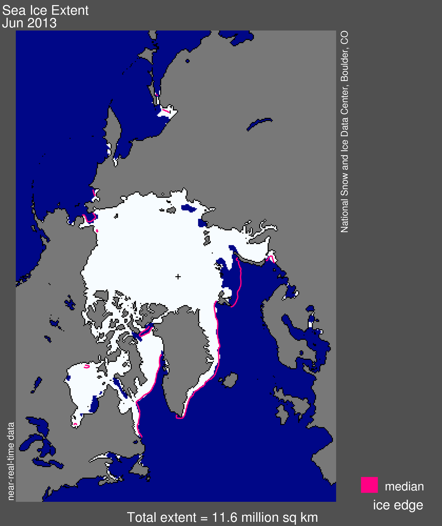
Figure 1. Arctic sea ice extent for June 2013 was 11.58 million square kilometers (4.47 million square miles). The magenta line shows the 1981 to 2010 median extent for that month. The black cross indicates the geographic North Pole. Sea Ice Index data. About the data
Credit: National Snow and Ice Data Center
High-resolution image
June is a transition period for Arctic sea ice as 24-hour daylight reigns, and melt reaches towards the North Pole. Thus it is an appropriate time for NSIDC to transition to a new 30-year baseline period, also called a “climate normal.” The satellite record is now long enough to allow NSIDC to match current National Ocean and Atmospheric Administration (NOAA) and World Meteorological Organization (WMO) standard baselines of 1981 to 2010 for weather and climate data. Full details of the changes and the implications for NSIDC sea ice statistics are described in the NSIDC Sea Ice Index.
Average sea ice extent for June 2013 was 11.58 million square kilometers (4.47 million square miles). This was 310,000 square kilometers (120,000 square miles) below the 1981 to 2010 average (the new baseline period) of 11.89 million square kilometers (4.59 million square miles). In comparison, the 1979 to 2000 period that we previously used averaged 12.16 million square kilometers (4.70 million square miles). June 2013 was 760,000 square kilometers (293,000 square miles) above the record low June extent in 2010.
Conditions in context

Figure 2a. The graph above shows Arctic sea ice extent as of June 30, 2013, along with daily ice extent data for five previous years. 2013 is shown in blue, 2012 in green, 2011 in orange, 2010 in pink, 2009 in navy, and 2008 in purple. The 1981 to 2010 average is in dark gray. Sea Ice Index data.
Credit: National Snow and Ice Data Center
High-resolution image

Figure 2b. The graph above shows Arctic sea ice extent as of June 30, 2013, along with daily ice extent data for 2012, the record low year, and both the new and old baseline average periods. The 1981 to 2010 average is shown by a dark gray line. The gray area around this average line shows the two standard deviation range of the 1981 to 2010 average. The 1979 to 2000 average is shown by a blue line. The light purple shading around this line shows the two standard deviation range of the 1979 to 2000 average.
Credit: National Snow and Ice Data Center
High-resolution image
Although the rate of ice loss increased toward the end of June, overall ice has retreated more slowly this summer compared to last summer, reflecting patterns of atmospheric circulation and air temperature. Average June temperatures at the 925 mb level were average to slightly below average over most of the Arctic Ocean, contrasting with above average temperatures over most of the surrounding land. This temperature pattern is associated with unusually low sea level pressure centered near the North Pole. This type of circulation pattern is known to slow the summer retreat of ice, not just because it fosters cool conditions, but also because the pattern of cyclonic (counterclockwise) winds tends to spread the ice out. An interesting regional aspect of this pattern is that on the heels of unusually cold spring conditions, the Alaska interior experienced some days of record high temperatures during June.
June 2013 compared to previous years

Figure 3. Monthly June ice extent for 1979 to 2013 shows a decline of 3.6% per decade relative to the 1981 to 2010 average.
Credit: National Snow and Ice Data Center
High-resolution image
Sea ice extent declined steadily through most of the month, in sharp contrast to last year when June experienced a record fast pace of sea ice retreat. There was a speed-up in ice loss toward the end of the month. Overall, extent dropped an average of 70,300 square kilometers (27,000 square miles) per day through the month, slightly higher than the 1981 to 2010 average.
June 2013 was the 11th lowest June in the 1979 to 2013 satellite record, 760,000 square kilometers (293,000 square miles) above the record low in 2010. The monthly trend is -3.6% percent per decade relative to the 1981 to 2010 average (also -3.6% per decade relative to the old 1979 to 2000 baseline).
An Arctic pre-conditioned for rapid summer ice loss?
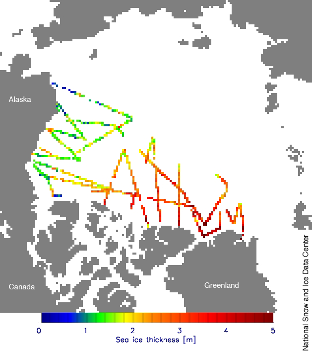
Figure 4. Data from NASA Operation IceBridge flights over the Arctic Ocean during March and April 2013 indicate thick ice along the Greenland coast (shown in reds), but thin ice north of Alaska (blues and greens).
Credit: National Snow and Ice Data Center/NASA Operation IceBridge
High-resolution image
Through most of June, we did not see the precipitous decline in ice extent that was observed in June 2012 and 2007 (the years with the lowest and second lowest September ice extent in the satellite record). However, the rate of ice loss did increase in late June. Ice cover this spring was very thin in parts of the Arctic, suggesting that large areas may soon start melting out completely. Much depends on whether the atmospheric circulation pattern seen in June persists through July.
NASA Operation IceBridge data collected during March and April indicated thick ice along the Greenland coast (5 meters, or 16 feet or more), but thin ice north of Alaska in the Beaufort and Chukchi seas, ranging from 1 to 1.5 meters (3 to 5 feet) in most areas and as low as 0.5 meters (approximately 2 feet) in others. These thin areas are quite likely refrozen leads, linked to the major fracturing events that occurred in the region during February and March. According to Andrew Shepherd at the University of Leeds, preliminary results from the European Space Agency CryoSat satellite suggest that the ice pack was 8% thinner in March 2013 compared to March 2012.
An ocean of small floes

Figure 5. High-resolution passive microwave data from AMSR2 on June 26, 2013 (left image) shows areas of low ice concentration near the North Pole, indicated in greens. Visible imagery from MODIS on June 27, 2013 (right image) of the inset area reveals a fractured ice surface with small floes.
Credit: University of Bremen/AMSR2; NASA/GSFC, Rapid Response
High-resolution image
High-resolution passive microwave concentration data from the Japan Aerospace Exploration Agency AMSR2 sensor, produced by the University of Bremen, indicate a highly unusual region of broken-up ice near the North Pole. Development of this low concentration ice may have been assisted by the cyclonic atmospheric pattern noted earlier.
While the AMSR2 image in Figure 5 suggests concentrations as low as 50%, visible imagery from the MODIS sensor on the NASA Aqua satellite indicate that AMSR2 is underestimating concentration, likely due to biases from surface melt.
Still, the MODIS data do confirm that the ice is highly fractured with numerous small floes. Such small floes are more easily melted from the sides and the bottom by ocean waters that are exposed to the 24-hour sunlight. It remains to be seen how many of these small floes will ultimately melt completely.

