June set another satellite-era record low for average sea ice extent, despite slower than average rates of ice loss. The slow rate of ice loss reflects the prevailing atmospheric pattern, with low pressure centered over the central Arctic Ocean and lower than average temperatures over the Beaufort Sea.
Overview of conditions
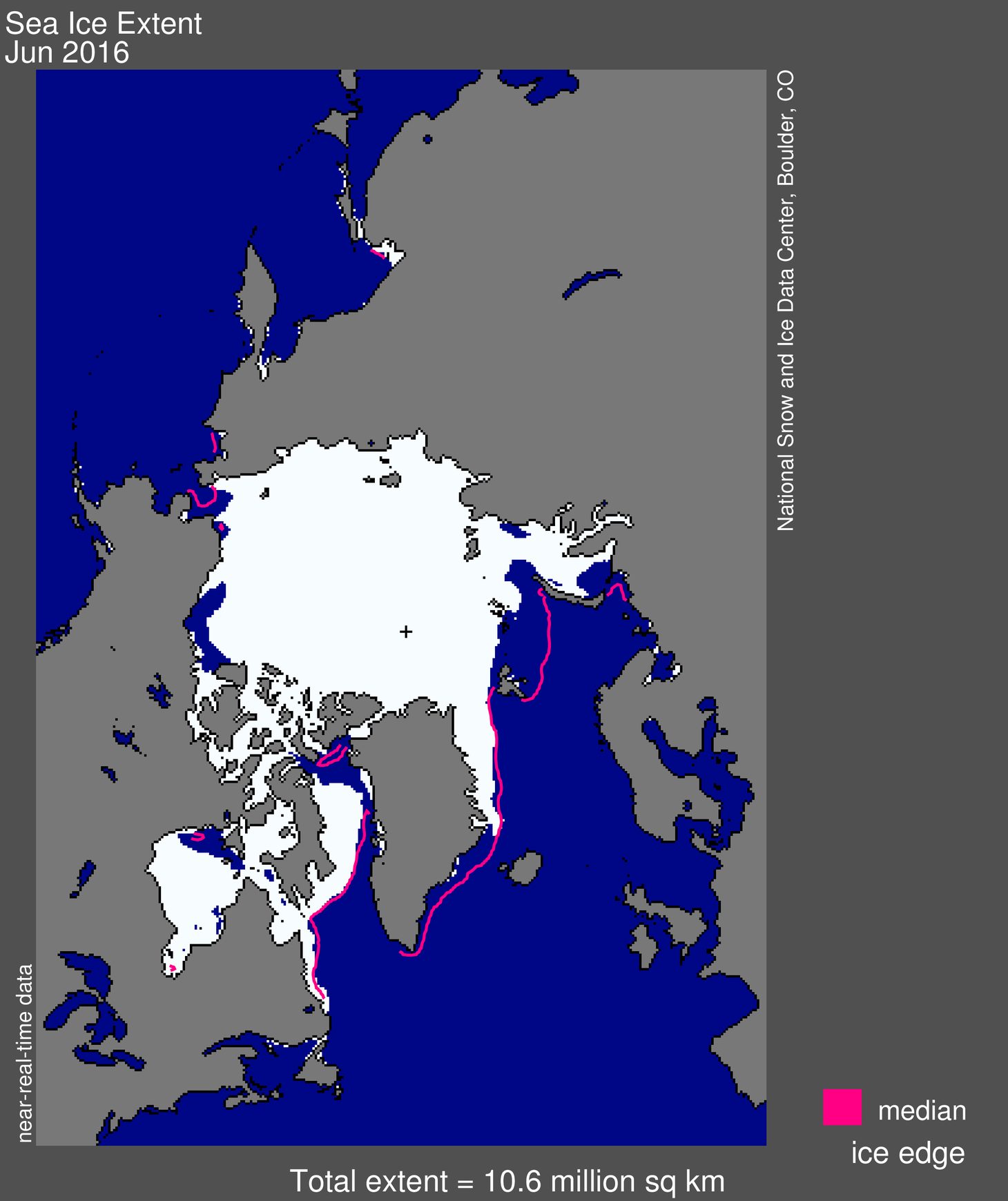
Figure 1. Arctic sea ice extent for June 2016 was 10.60 million square kilometers (4.09 million square miles). The magenta line shows the 1981 to 2010 median extent for that month. The black cross indicates the geographic North Pole. Sea Ice Index data. About the data
Credit: National Snow and Ice Data Center
High-resolution image
Arctic sea ice extent during June 2016 averaged 10.60 million square kilometers (4.09 million square miles), the lowest in the satellite record for the month. So far, March is the only month in 2016 that has not set a new record low for Arctic-wide sea ice extent (March 2016 was second lowest, just above 2015). June extent was 260,000 square kilometers (100,000 square miles) below the previous record set in 2010, and 1.36 million square kilometers (525,000 square miles) below the 1981 to 2010 long-term average.
Sea ice extent remains below average in the Kara and Barents seas, as it has throughout the winter and spring. Despite lower than average temperatures over the Beaufort Sea, sea ice extent there remains below average, and was the second lowest extent for the month of June during the satellite data record.
Conditions in context
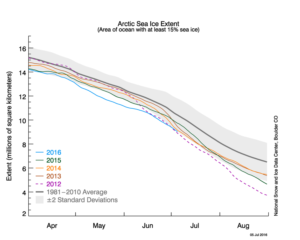
Figure 2a. The graph above shows Arctic sea ice extent as of July 5, 2016, along with daily ice extent data for four previous years. 2016 is shown in blue, 2015 in green, 2014 in orange, 2013 in brown, and 2012 in purple. The 1981 to 2010 average is in dark gray. The gray area around the average line shows the two standard deviation range of the data. Sea Ice Index data.
Credit: National Snow and Ice Data Center
High-resolution image
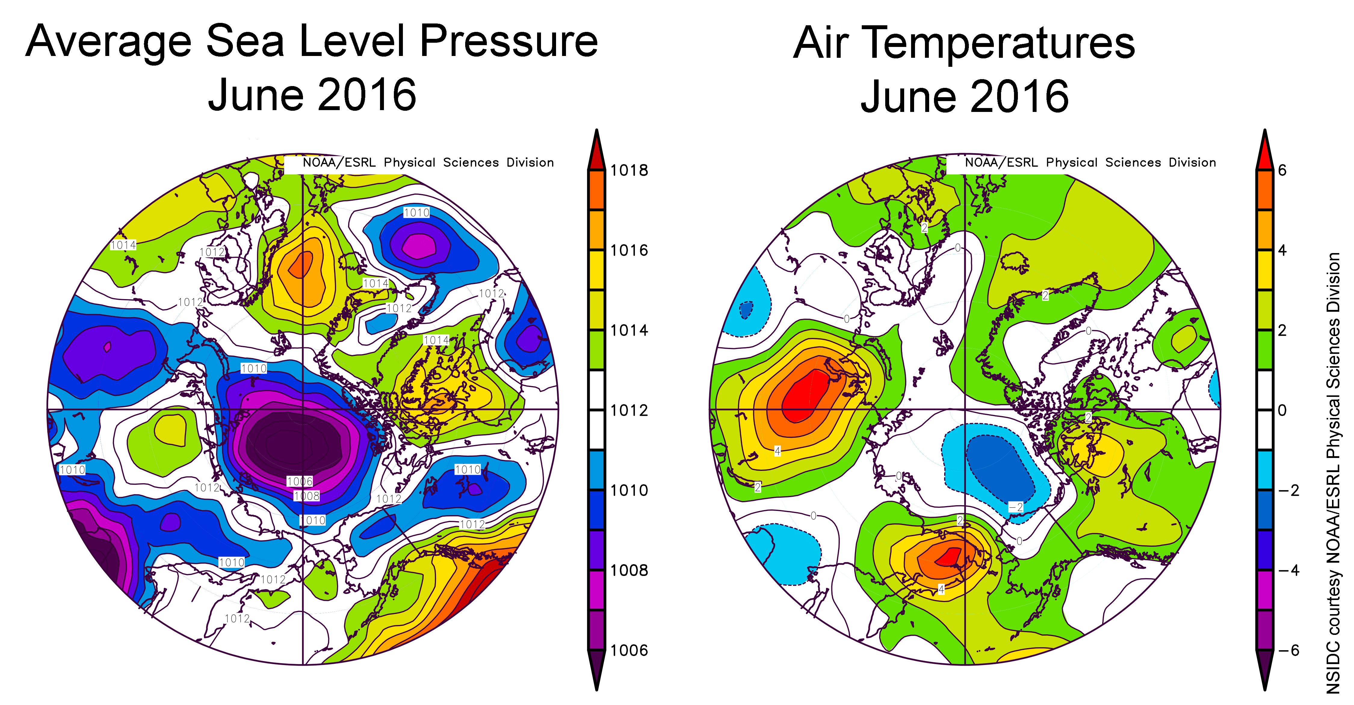
Figure 2b. The map of sea level pressure averaged for the month of June 2016 (left) shows low pressure over the central Arctic Ocean. The map of air temperatures at 925 hPa for June 2016 compared to the 1981 to 2010 long-term average (right) shows cool conditions over the Beaufort Sea.
Credit: NSIDC courtesy NOAA/ESRL Physical Sciences Division
High-resolution image
The average rate of ice loss during June 2016 was 56,900 square kilometers (22,000 square miles) per day, but was marked by two distinct regimes. First, there was a period of slow loss during June 4 to 14 of only 37,000 square kilometers (14,000 square miles) per day. This was followed by above average rates (74,000 square kilometers, or 29,000 square miles) for the rest of the month. For the month as a whole, the rate of loss was close to average (53,600 square kilometers per day). The slow ice loss during early June was a result of a significant change in the atmospheric circulation. May was characterized by high surface pressure over the Arctic Ocean, a basic pattern that has held since the beginning of the year. However, June saw a marked shift to low pressure over the central Arctic Ocean. This type of pattern is known to inhibit ice loss. A low pressure pattern is associated with more cloud cover, limiting the input of solar energy to the surface, as well as generally below average air temperatures. However, in June 2016, it was only in the Beaufort Sea where air temperatures at the 925 hPa level were distinctly below average (about 2 degrees Celsius below average, or 4 degrees Fahrenheit). The change in circulation also shifted the pattern of ice motion. In general, winds associated with such a low pressure pattern will tend to spread the ice out (that is, cause the ice to diverge).
June 2016 compared to previous years
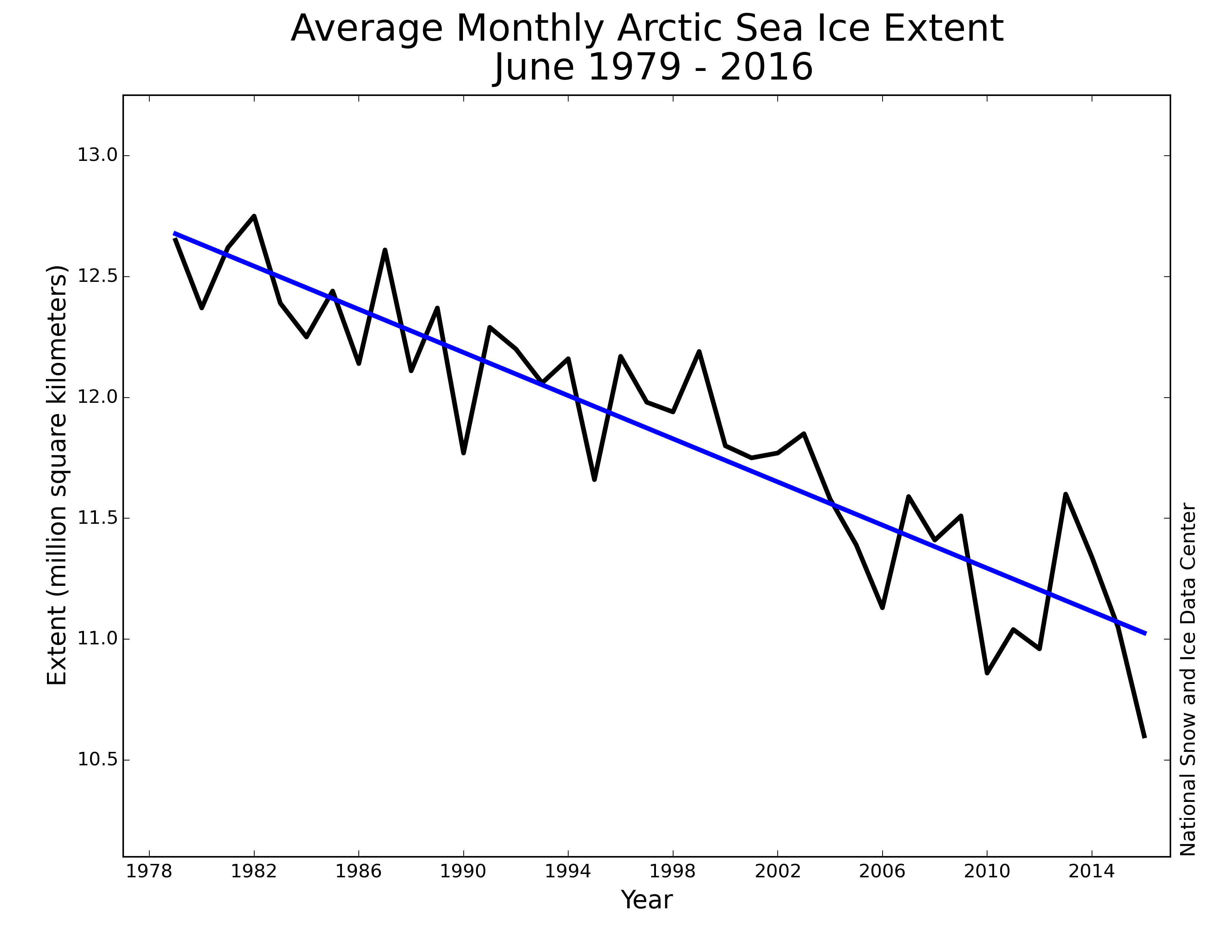
Figure 3. Monthly June ice extent for 1979 to 2016 shows a decline of 3.7% per decade.
Credit: National Snow and Ice Data Center
High-resolution image
Through 2016, the rate of decline for the month of June is 44,600 square kilometers (17,200 square miles) per year, or 3.7 percent per decade. June extent remained below 2012 levels throughout the month, but it was above the 2010 extent for several days. 2010 had the lowest extent for several days during June.
View from above
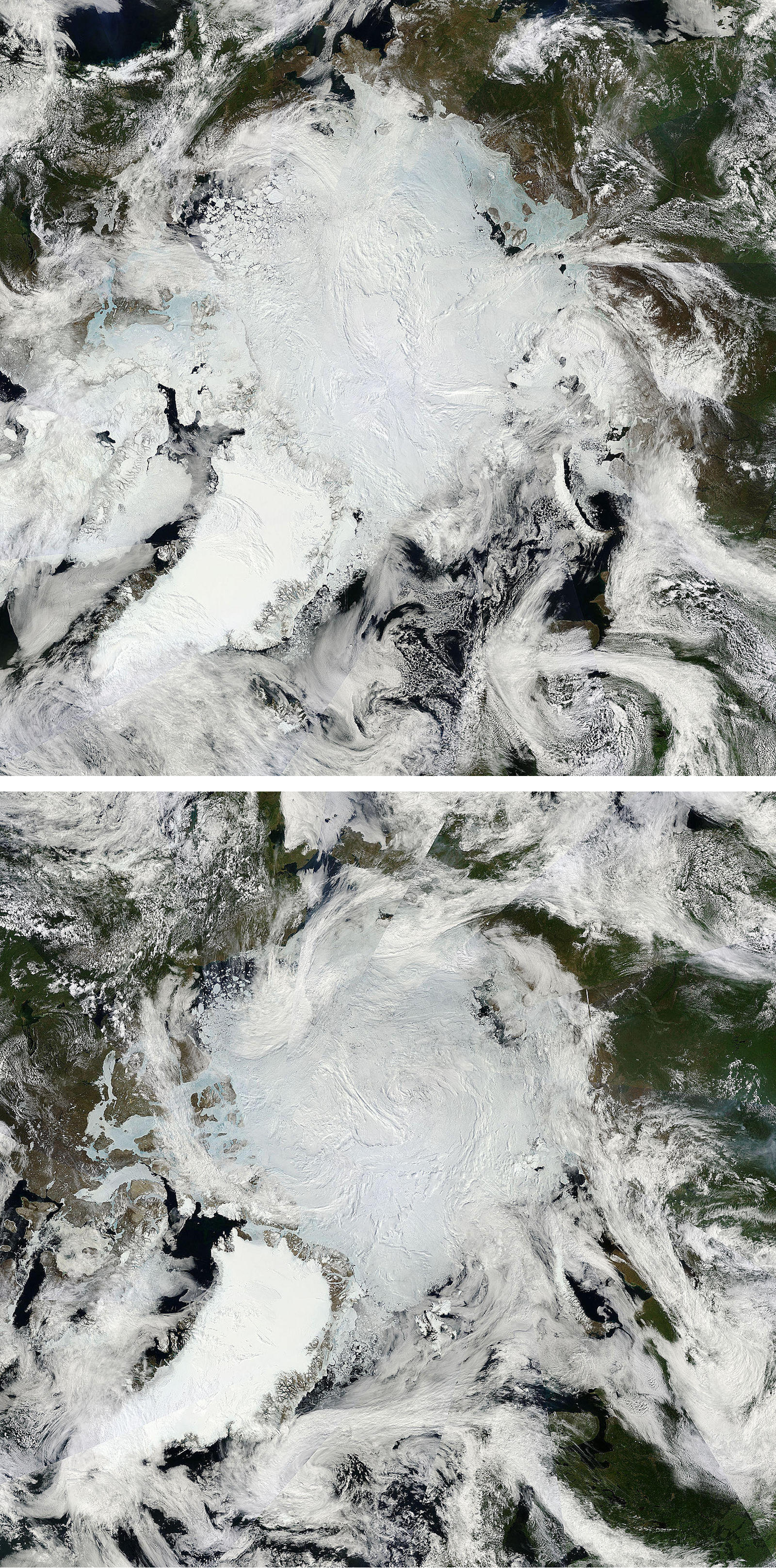
Figure 4. MODIS composite images for June 9, 2016 (top) and June 28, 2016 (bottom) show the seasonal progression of surface melting and darkening of the ice surface.
Credit: Land Atmosphere Near-Real Time Capability for EOS (LANCE) System, NASA/GSFC
High-resolution image
The Moderate Resolution Imaging Spectroradiometer (MODIS) instruments on the NASA Aqua and Terra satellites provide multiple views each day of the Arctic, and in summer the entire region is sunlit. Two mosaics for June 9 and June 28 show the seasonal progression in surface melting and darkening of the sea ice; the blue-green areas where surface ponding is present; and the movement of large sea ice floes in the Beaufort Sea. On June 9, the ponds are most evident in the Laptev Sea off the coast of Siberia; on June 28, the ponds are most evident in the Canadian Archipelago.
A quick look at sea ice thickness fields
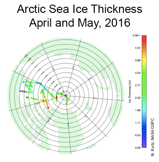
Figure 5. Sea ice thickness from April and May 2016 from Operation IceBridge. Image courtesy Nathan Kurtz, NASA Goddard.
Credit: N. Kurtz, NASA Goddard Space Flight Center
High-resolution image
Results from NASA’s Operation IceBridge aircraft missions conducted during late April and early May indicate that ice thicknesses from the Alaskan coast of the Beaufort Sea up to the North Pole were generally in the 2 to 3 meter range (7 to 10 feet), indicative of multiyear ice. However, substantial variations were found along the flight transects with several locations showing an ice thickness of 1.5 meters (5 feet) or less, indicative of first-year ice, while in other locations thicknesses were over 5 meters (16 feet), corresponding to either fairly thick multiyear ice or ridged first-year ice. This substantial variation is representative of a broken up and variegated ice pack with thick multiyear floes interspersed with thinner first-year ice.
The first-year thicknesses were found to be generally thinner than is typical at the end of winter, which is consistent with the usually high temperatures characterizing last winter. Very thin ice (less than 0.5 meters, or 1.6 feet) was found in places near the Alaskan coast, where leads opened up fairly late in the ice growth season. The IceBridge results are generally in agreement with the ice thickness surveys conducted in early April by researchers from York University, and with CryoSat-2 thickness maps discussed in our previous post.
Sea Ice Outlook
Each summer the Sea Ice Prediction Network (SIPN) requests forecasts of the September average sea ice extent. Requests are made in June July and August. This year, thirty contributions to the June Sea Ice Outlook were received, employing a variety of methods, including statistical models, dynamical models, and informal polls. The median prediction for this year’s September sea ice extent is 4.28 million square kilometers (1.65 million square miles), similar to the extent observed in 2007. Dynamical models predict 4.58 million square kilometers (1.77 million square miles), compared to the slightly lower overall median extent prediction of 4.28 million square kilometers (1.65 million square miles) from statistical models. The lowest median extent comes from the heuristic contributions (4.0 million square kilometers, or 1.5 million square miles). Only one forecast points towards a new record low for 2016.
Antarctic sea ice
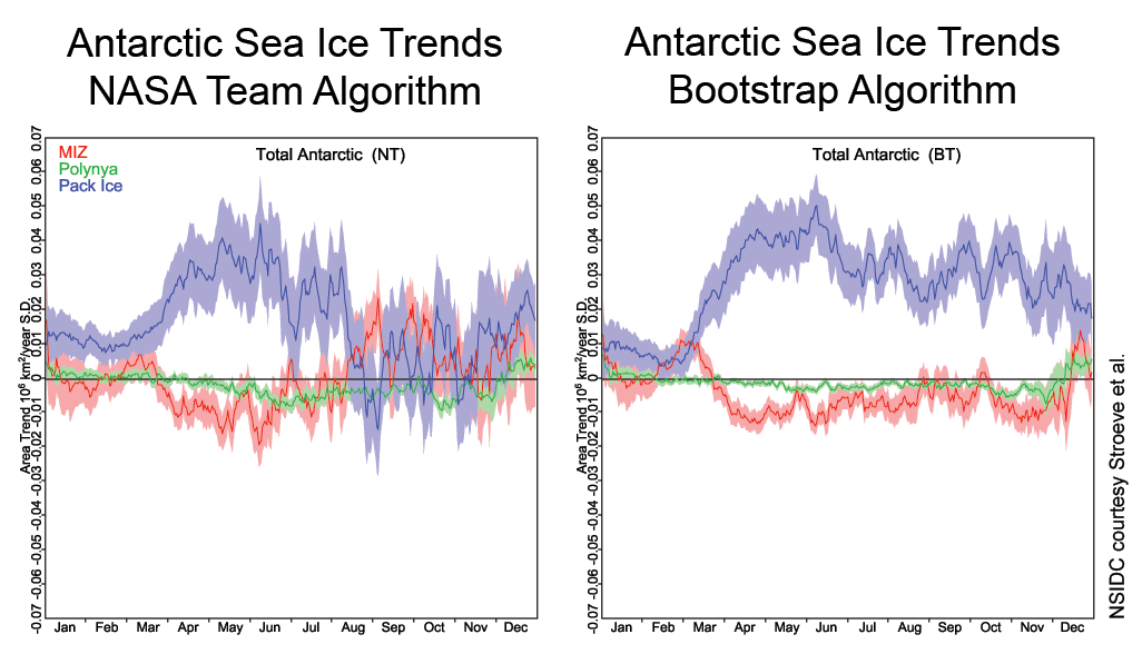
Figure 6. Circumpolar Antarctic trends from 1979 to 2014 in the consolidated pack ice (blue), the marginal ice zone (red) and coastal polynyas (green) from the NASA Team sea ice algorithm (left) and the Bootstrap algorithm (right).
Credit: National Snow and Ice Data Center, Stroeve et al.
High-resolution image
Antarctic sea ice extent continues to track at near average levels, in sharp contrast to the previous two winters, which were above average. While the total ice extent in the Antarctic shows a small positive trend, particularly during the cold season, whether or not the total mass of the ice has changed depends on how much of the pack ice consists of consolidated ice, the extent of the marginal ice zone (the outer edge of the ice pack, which is lower in ice concentration), and coastal polynyas (open water areas near the coast). The marginal sea ice zone and the coastal polynyas have important biological implications. These are key regions for phytoplankton productivity and krill abundance that in turn feed Antarctic sea birds and nektonic fauna (things that swim).
A new study looks at how these regions are changing using two sea ice concentration algorithms distributed by NSIDC. While the algorithms give similar trends in the overall sea ice extent, they differ in terms of whether or not the sea ice cover is becoming more compacted (i.e., the consolidated ice pack is increasing in extent) or if the marginal ice zone is expanding (Figure 6). When sea ice is is growing seasonally, both algorithms indicate that it is due to an expansion of the consolidated ice pack, whereas during winter and spring, one measurement method (the NASA Team algorithm) finds the marginal ice zone is also expanding as well, and the other measurement (Bootstrap algorithm) shows no significant trend in the marginal ice. The algorithms also differ in how much of the total ice pack consists of pack ice or the marginal ice, with the NASA Team algorithm having on average twice as large of a marginal ice zone as the Bootstrap algorithm. As well, the NASA Team algorithm is known to underestimate ice concentration in the Antarctic. This highlights the need for further validation of sea ice concentrations derived from passive microwave satellite data.
New Sea Ice Index version
As part of our quality control process, the Sea Ice Index, which supplies sea ice extent and concentration values, has been updated to Version 2. Changes include using the most recently available version of the Sea Ice Concentrations from Nimbus-7 SMMR and DMSP SSM/I-SSMIS Passive Microwave Data that provide final sea ice concentration data. The version update also adjusted three procedures in the Sea Ice Index processing routine that affected both the near-real-time data and the final data. These four updates affect different portions of the Sea Ice Index time series. Because of these updates, minor changes in some of the ice extent and area numbers will be seen. However, these changes are almost all quite small and do not alter current conclusions about Arctic or Antarctic sea ice conditions. More information on Version 2 is available in the Sea Ice Index documentation.
Reference
Stroeve, J. C., Jenouvrier, S., Campbell, G. G., Barbraud, C., and Delord, K. 2016, in review. Mapping and assessing variability in the Antarctic Marginal Ice Zone, the pack ice and coastal polynyas. The Cryosphere Discuss., doi:10.5194/tc-2016-26.

