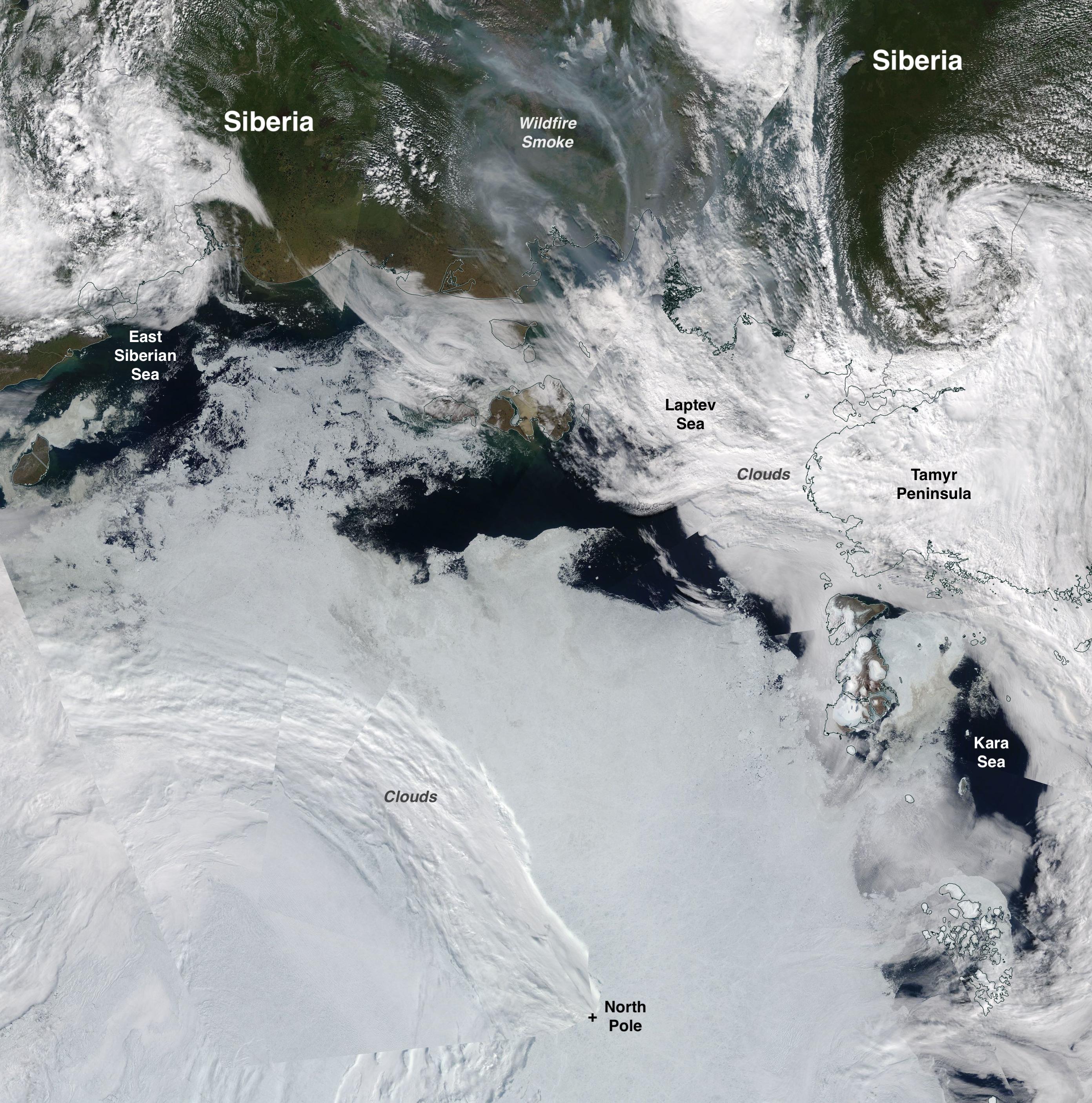
While the Arctic summer is waning, sea ice extent continues to drop. In early August, ice-free pockets began to develop in the Beaufort and Chukchi Seas and expanded steadily through the first half of the month.

Overview of conditions

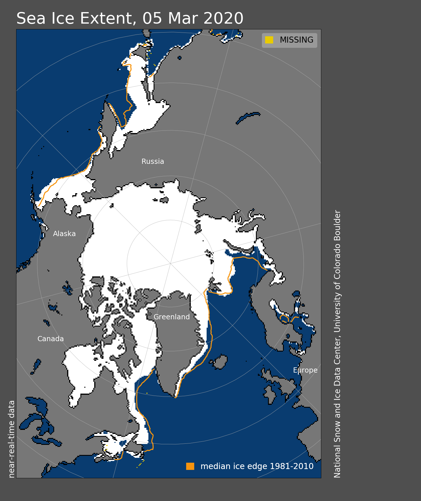
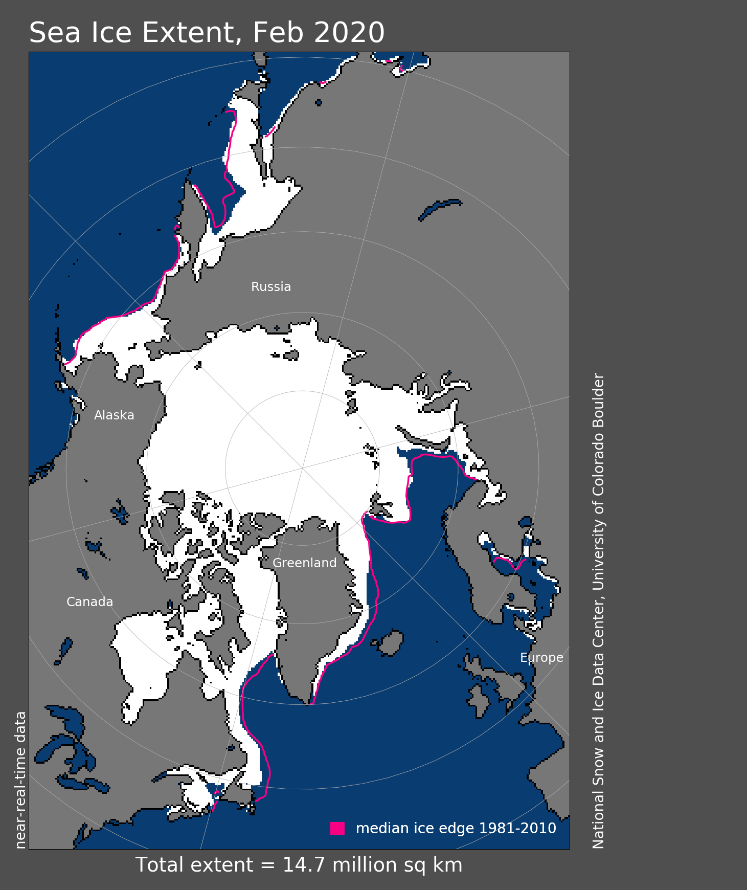
Figure 1a. Arctic sea ice extent for August 17, 2020 was 5.15 million square kilometers (1.99 million square miles). The orange line shows the 1981 to 2010 average extent for that day. Sea Ice Index data. About the data

Credit: National Snow and Ice Data Center
High-resolution image

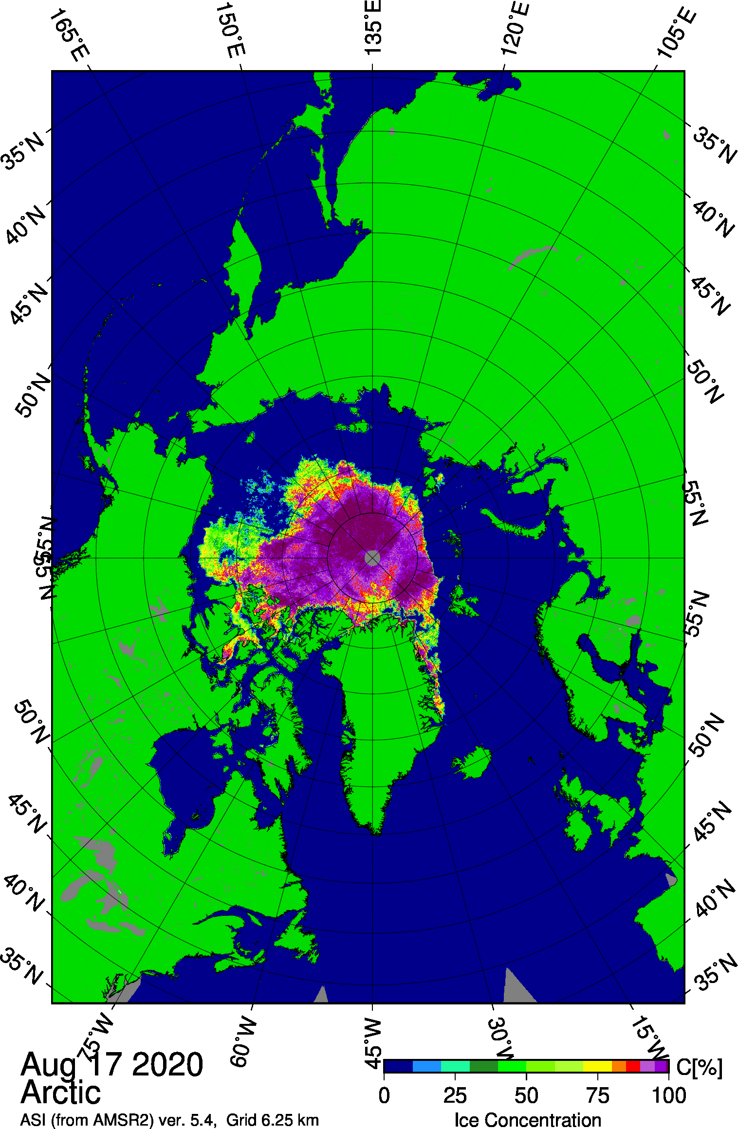
Figure 1b. This Japan Aerospace Exploration Agency (JAXA) Advanced Microwave Scanning Radiometer 2 (AMSR2) image shows sea ice concentration in the Arctic Ocean on August 17, 2020, highlighting the openings of sea ice north of Alaska within the Beaufort and Chukchi Seas.

Credit: University of Bremen
High-resolution image

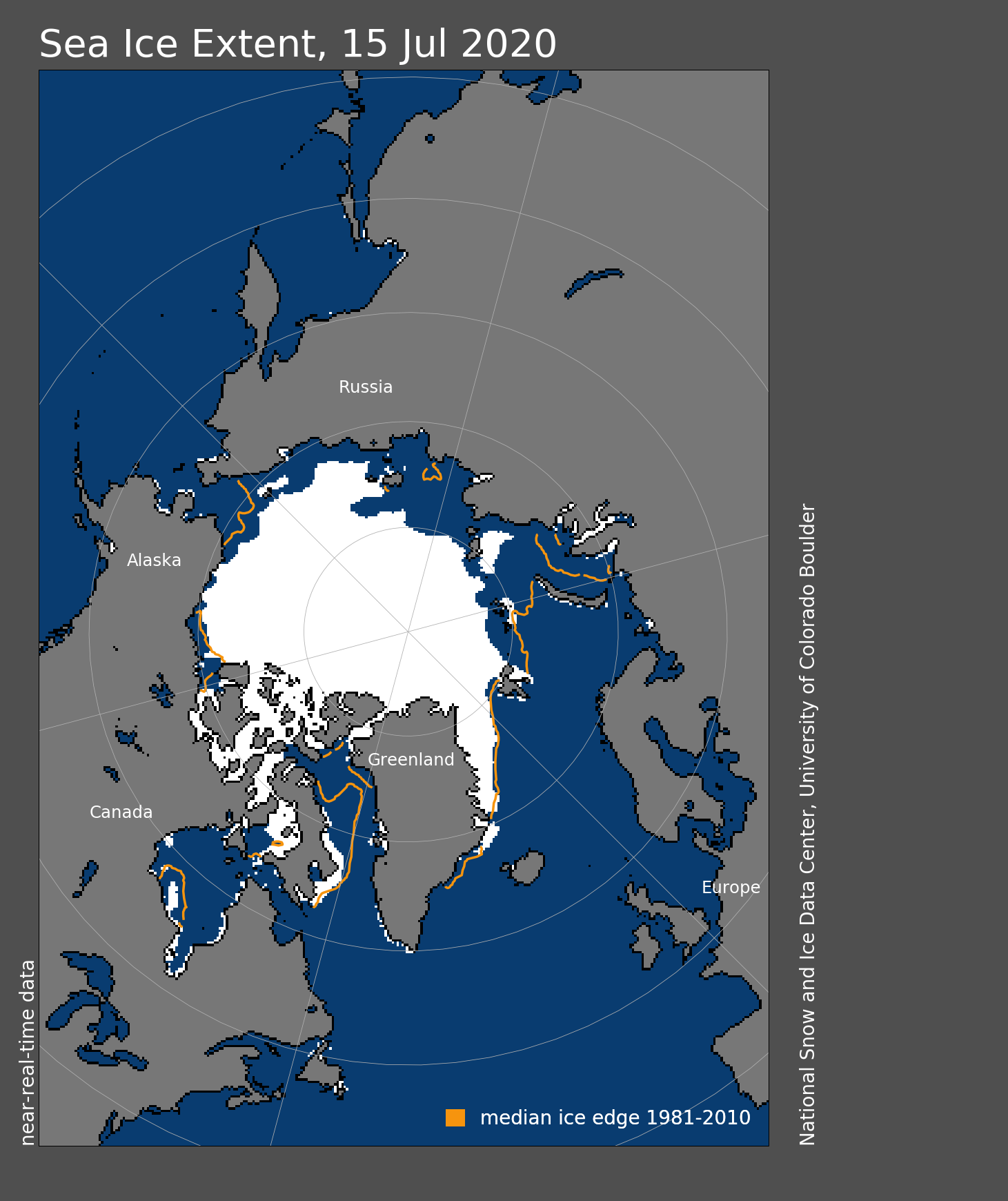
Sea ice extent stood at 5.15 million square kilometers (1.99 million square miles) on August 17, essentially tied with 2007 for the third lowest extent for the date since the satellite record began in 1979 (Figure 1a). The August 17 extent was lower only in 2012 and 2019. The most notable feature during the first half of August was the development of substantial openings of the sea ice north of Alaska within the Beaufort and Chukchi Seas. This may be related to the mid-July storm that passed and spread out the ice cover, creating openings in the sea ice.

The reduced concentration patches and initial openings were first observed in higher-resolution Japan Aerospace Exploration Agency (JAXA) Advanced Microwave Scanning Radiometer 2 (AMSR2) fields from the University of Bremen (Figure 1b). By the middle of the month, the ice-free areas had greatly expanded. Meanwhile, another open water patch developed north of the Mackenzie River delta. Persistent offshore winds have also moved the pack ice edge northward from the northern Greenland and Ellesmere coasts.

The Northern Sea Route has been open for a few weeks. The Northwest Passage appears to be mostly ice-free with a little ice remaining within Victoria Strait. The deeper Parry Channel still contains a substantial amount of sea ice and will likely not open this year.

Conditions in context

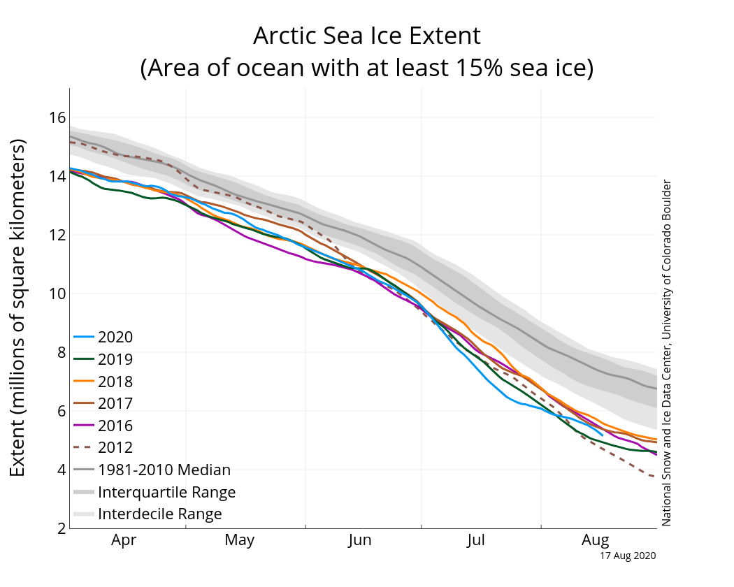
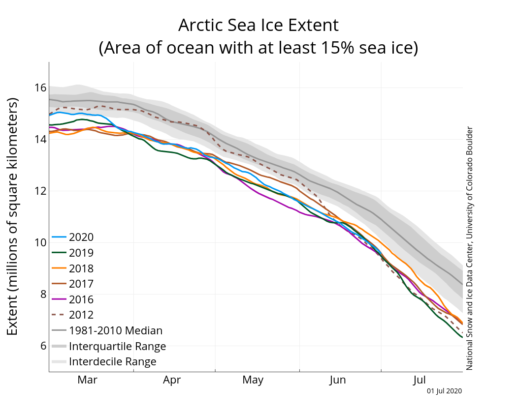
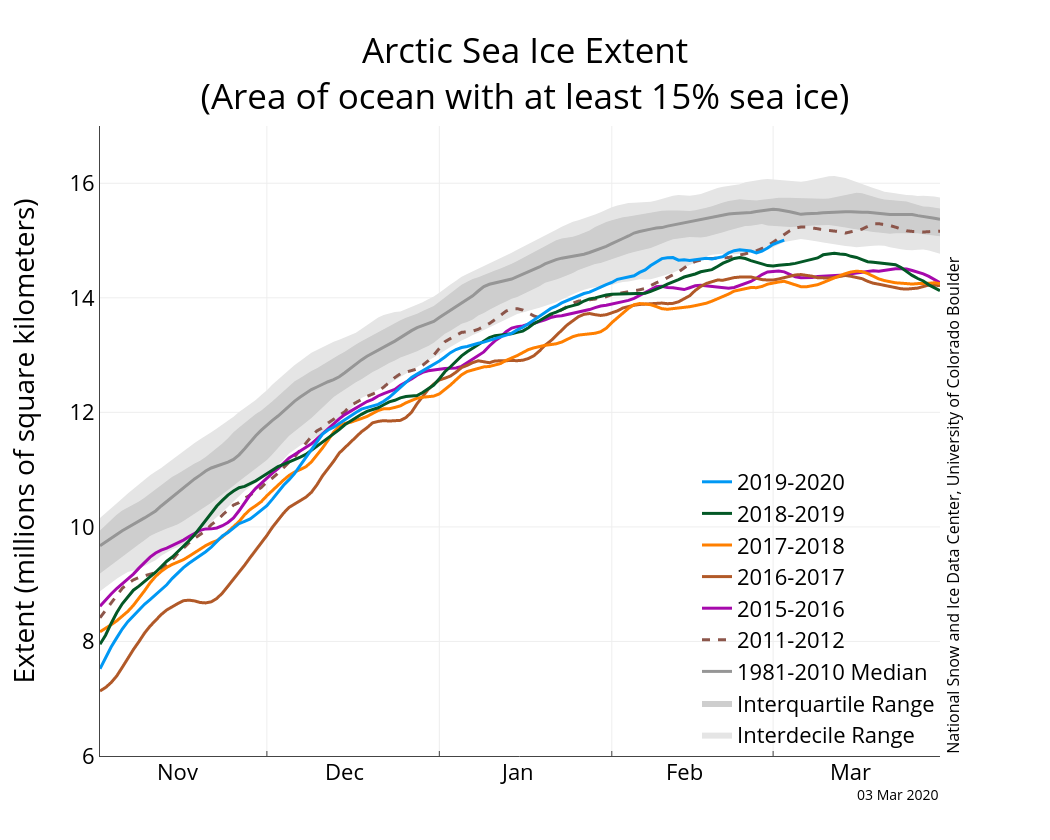
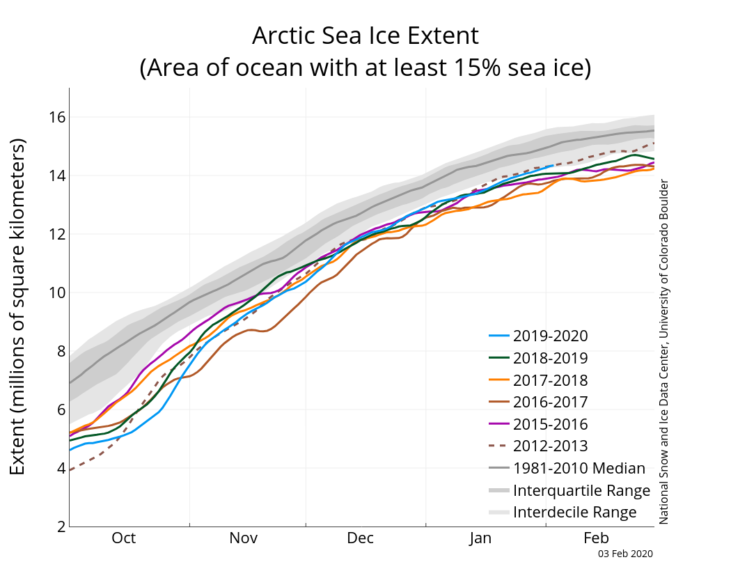
Figure 2a. The graph above shows Arctic sea ice extent as of August 17, 2020, along with daily ice extent data for four previous years and the record low year. 2020 is shown in blue, 2019 in green, 2018 in orange, 2017 in brown, 2016 in purple, and 2012 in dashed brown. The 1981 to 2010 median is in dark gray. The gray areas around the median line show the interquartile and interdecile ranges of the data. Sea Ice Index data.

Credit: National Snow and Ice Data Center
High-resolution image

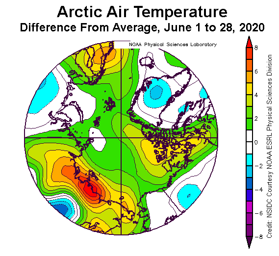
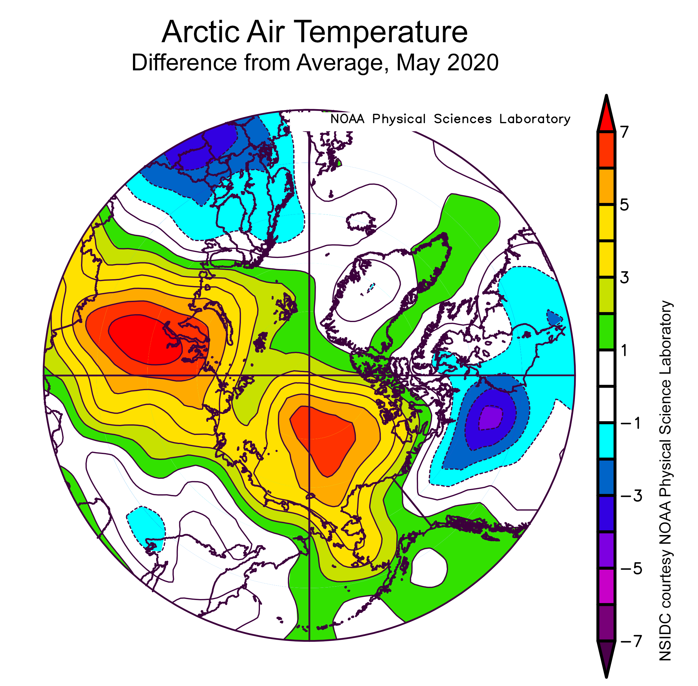
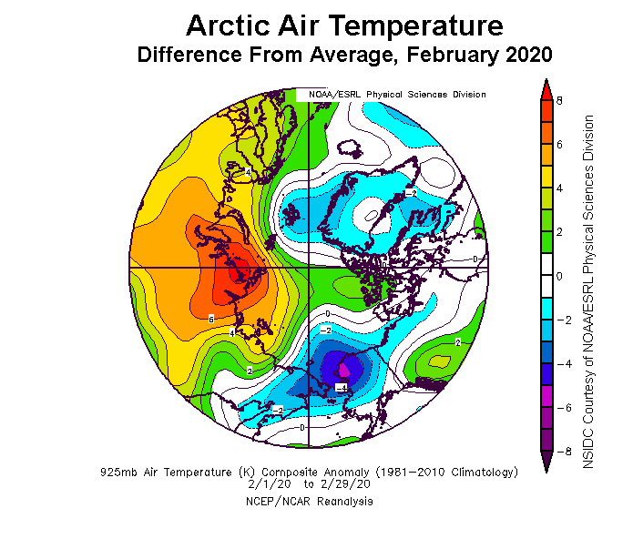
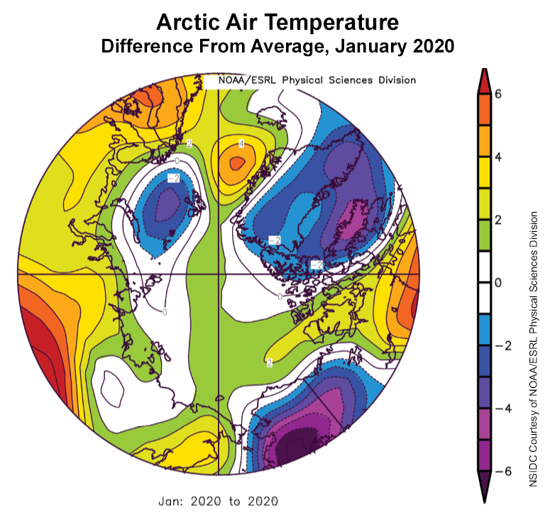
Figure 2b. This plot shows the departure from average air temperature in the Arctic at the 925 hPa level, in degrees Celsius, from August 1 to 15, 2020. Yellows and reds indicate higher than average temperatures; blues and purples indicate lower than average temperatures.

Credit: NSIDC courtesy NOAA Earth System Research Laboratory Physical Sciences Division
High-resolution image

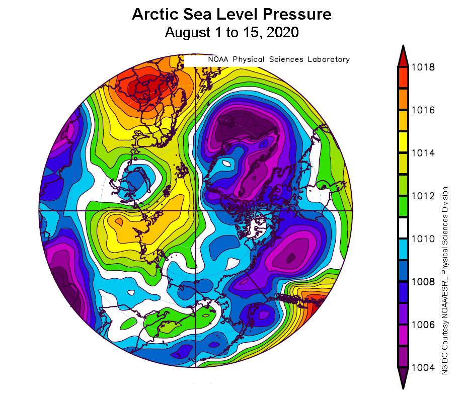
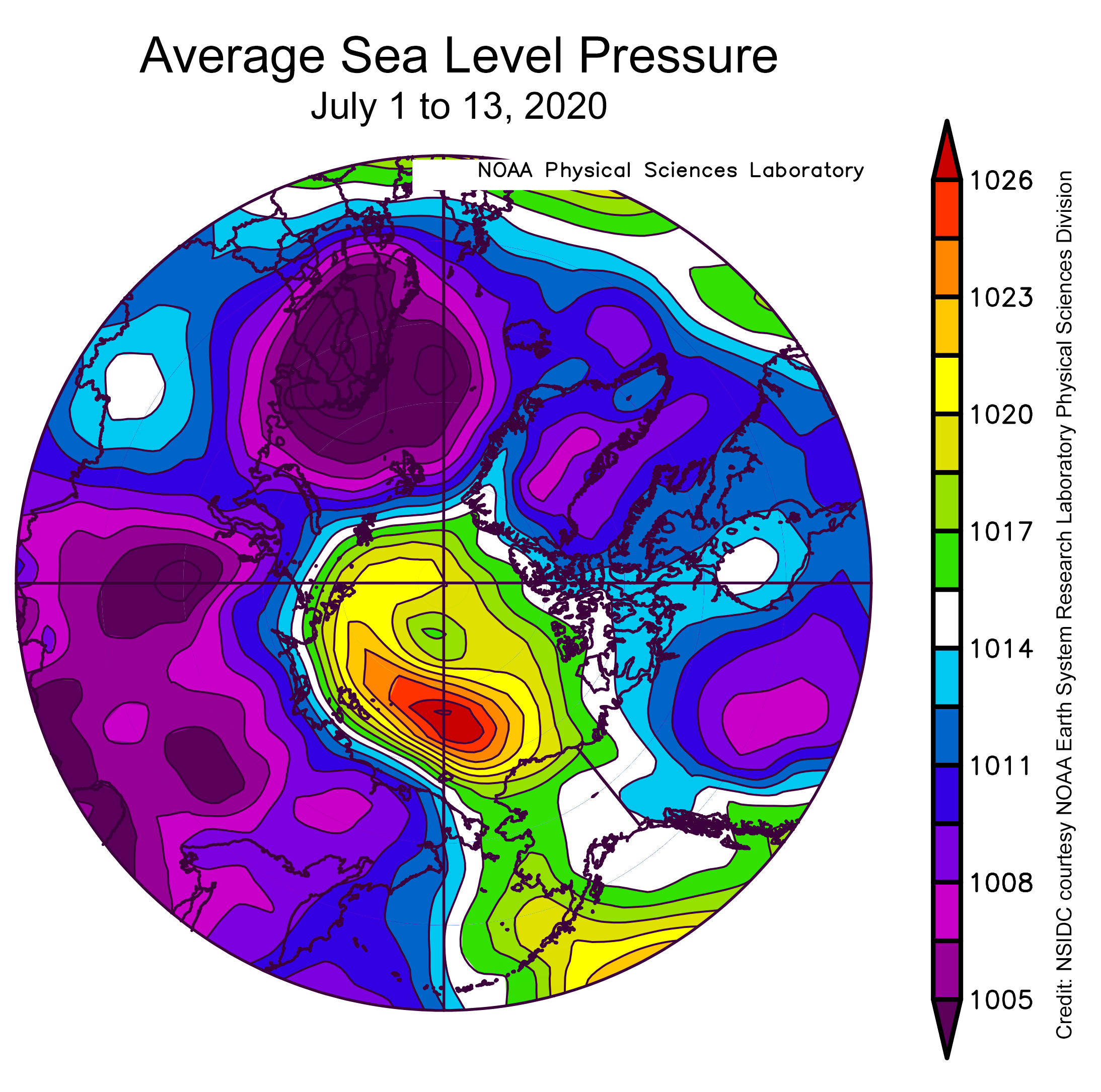
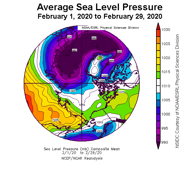
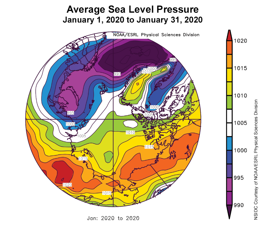
Figure 2c. This plot shows average sea level pressure in the Arctic in millibars (hPa) from August 1, 2020 to August 15, 2020. Yellows and reds indicate high air pressure; blues and purples indicate low pressure.

Credit: NSIDC courtesy NOAA Earth System Research Laboratory Physical Sciences Division
High-resolution image

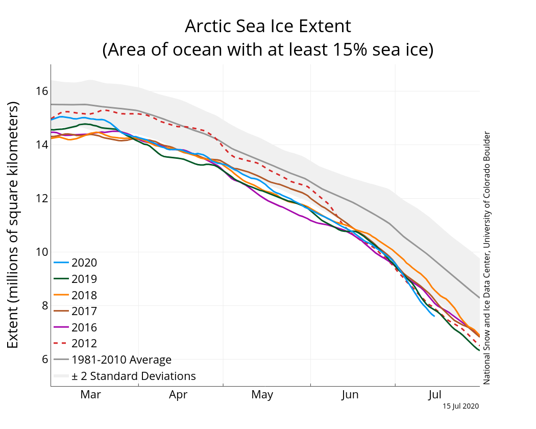
From July 27 through August 8, 2020, extent declined 470,000 square kilometers (181,000 square miles), which is less than half of the average 1981 to 2020 extent loss of 950,000 square kilometers (367,000 square miles) during the same period (Figure 2a). After August 8, the rate of loss increased again due in part to melt in the Beaufort and Chukchi Seas, though the loss rate was still slower than average.

As assessed from August 1 to 15, air temperatures at the 925 mb level (about 2,500 feet above sea level) were above average over much of the Arctic Ocean, with air temperatures up to 7 degrees Celsius (13 degrees Fahrenheit) above average over the North Pole. Temperatures were 1 to 3 degrees Celsius (2 to 5 degrees Fahrenheit) below average in the East Siberian Sea region (Figure 2b). The atmospheric circulation was characterized by generally high pressure on the Eurasian side of the Arctic and low pressure on the North American side (Figure 2c).

2020 Arctic sea ice minimum forecasts

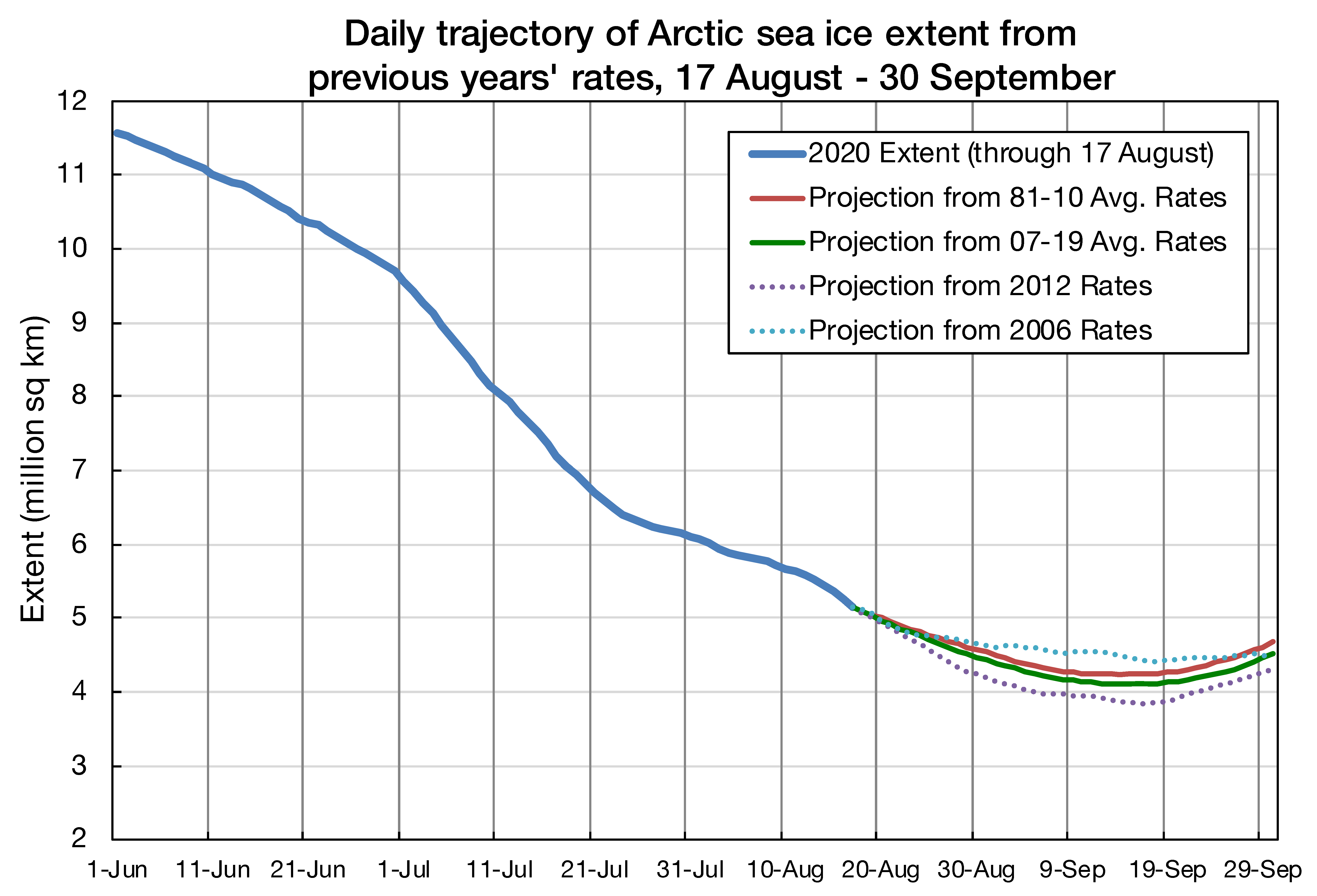
Figure 3. This figure show Arctic sea ice extent projections using data through August 17, 2020. These projections include the 2020 minimum and September 2020 average extent. These are based on the average loss rates for the years 2007 to 2019. The variation in the projection decreases for later dates because there is less time for variation before the end of the melt season.

Credit: National Snow and Ice Data Center
High-resolution image

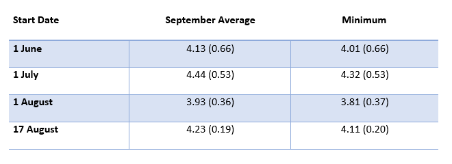
Table 1. This table shows a projection of Arctic sea ice extent for the September average and the daily minimum starting from June 1, July 1, August 1, and August 17, 2020. The projection is based on the average of the 2007 to 2019 estimates and the standard deviation range is in parentheses. Units are in millions of square kilometers.

Credit: National Snow and Ice Data Center
High-resolution image

The end of the summer melt season, when the Arctic sea ice extent reaches its seasonal minimum, is likely about three to four weeks away. Over the last several years, there has been a community effort, called the Sea Ice Outlook, to submit seasonal projections of the September monthly average extent and the daily seasonal minimum. One submission by Arctic Sea Ice News & Analysis (ASINA) team member Walt Meier uses ice extent loss rates from previous years to project this year’s ice loss through the end of summer. Projections of the minimum and September average extent are submitted using data through the beginning of June, July, and August as starting points. Another projection with data through August 17 is included here to provide a further update (Figure 3 and Table 1). The projections are based on the average loss rates for the years 2007 to 2019. The variation in the projection decreases for later dates because there is less time before the end of the melt season. Note how the projections have seesawed up and down from June through mid-August. This is a result of the changes in the extent loss rates from one period to the next; it highlights how strongly weather conditions affect the ice loss through the summer, as well as the influence of thickness on how fast ice is melted away.

Another projection from National Snow and Ice Data Center scientist Andy Barrett, using a probabilistic method developed by our former colleague Drew Slater, projects a September average extent of 4.48 million square kilometers (1.73 million square miles), which is slightly higher than the Meier method prediction.

Past ice-free Arctic Oceans

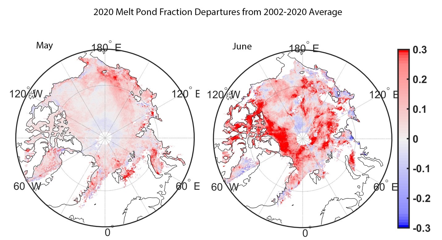
Climate models are projecting that under continued warming trends, the Arctic Ocean may become substantially ice-free during the summer within the next 30 years. Such a state would be unprecedented for at least thousands of years. However, such conditions may have existed during the Last Interglacial (LIG) period, about 130,000 to 116,000 years before present, when summer Arctic air temperatures were 4 to 5 degrees Celsius (7 to 9 degrees Fahrenheit) above pre-industrial levels. Previous model simulations were unable to capture the reconstruction of LIG Arctic temperatures, and a likely cause was a simplified treatment of sea ice that did not represent the influence of melt ponds on summer sea ice loss. The latest version of the UK Hadley Centre Global Environment Model version 3 (HadGEM3) climate model includes more complex characterization of melt ponds. In a recent paleoclimate study, this model was able to reproduce the reconstructed estimates of summer Arctic air temperatures during the LIG. This supports previous studies showing that melt pond formation is a key factor in the loss of summer sea ice because formation of melt ponds earlier in the season results in more absorption of solar energy through the summer and therefore more ice melt. ASINA team member Julienne Stroeve is a co-author on the study.

Farewell to the Milne Ice Shelf

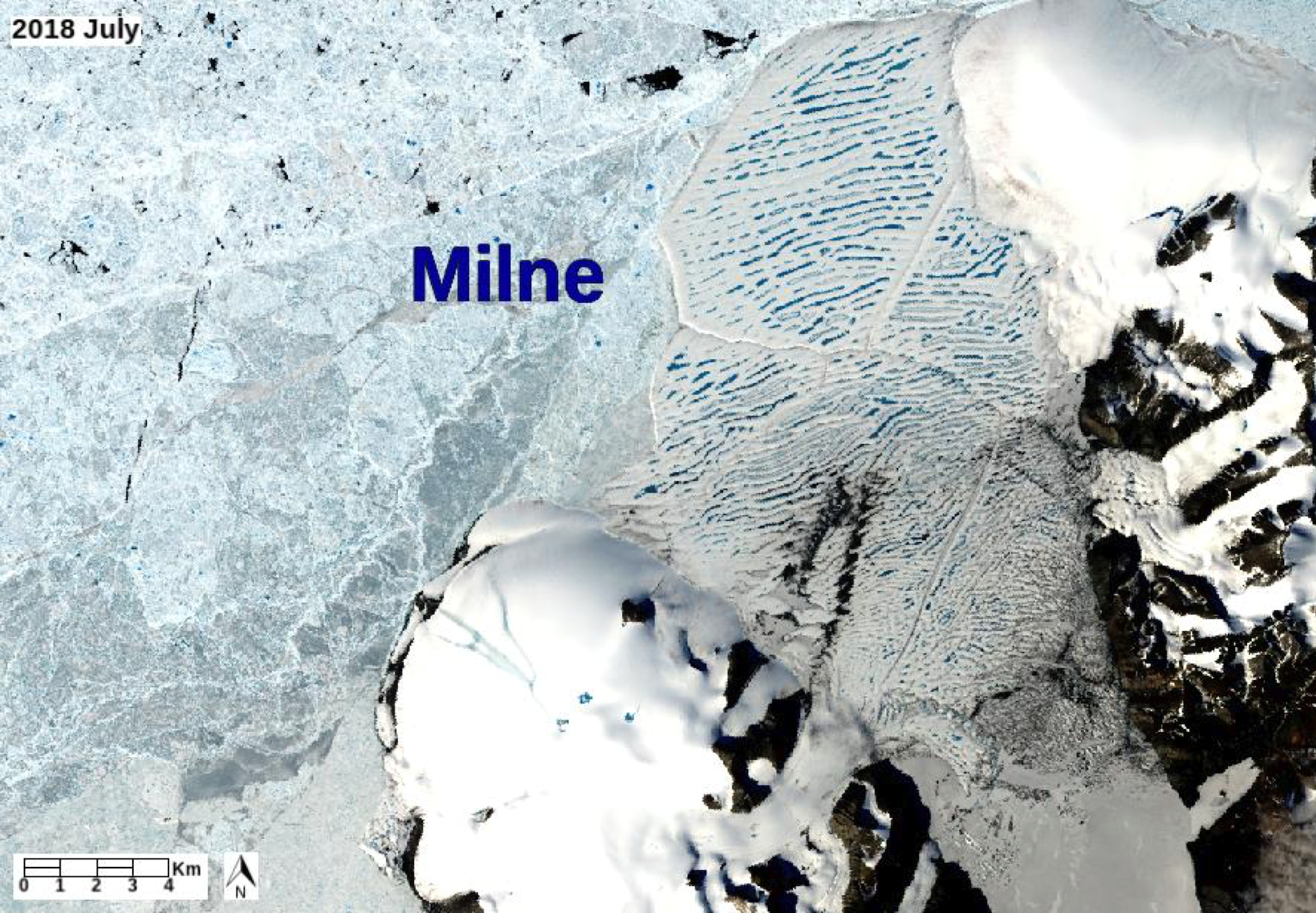
Figure 4. This NASA Landsat 8 true color image shows the former extent of the Milne Ice Shelf on Ellesmere Island in Nunavut, Canada, on July 23, 2018. It was acquired with off-nadir pointing of the satellite. The shelf is covered with linear blue lakes of meltwater that collect in the gently folded (corrugated) surface. In the upper left is the Arctic Ocean covered by perennial sea ice.

Credit: NASA
High-resolution image

Another recent notable event in the Arctic was the calving of a large area of the Milne Ice Shelf off Ellesmere Island in Nunavut, Canada, in late July. The Milne Ice Shelf had been Canada’s last intact Arctic ice shelf. A piece of the shelf measuring about 81 square kilometers (31 square miles), which made up about 43 percent of the total ice shelf area, broke off on July 30 and 31. Warm air temperatures and offshore winds likely triggered the ice shelf collapse. Offshore winds move the perennial sea ice cover north from the coast, reducing the compressive forces that hold the shelf in, and potentially contribute to basal melting of the ice by allowing solar energy to warm the upper ocean layer. Polar explorer Robert Peary discovered the Canadian Arctic ice shelves, once a single 9,000-square kilometer (3,475-square mile) sheet, in 1902. Although evidence from seal remains and driftwood suggests they were thousands of years old, they have dwindled dramatically and now comprise of only a few small ice-covered fragments in inlets along the northernmost coast of Canada.

Rest in peace, Koni Steffen

Former Cooperative Institute for Research in Environmental Sciences director Konrad Steffen passed away on August 8, 2020, while conducting field work on the Greenland Ice Sheet. He will be missed. Photo courtesy of CIRES/CU Boulder.

As has been widely reported, the polar climate community suffered a huge loss in the tragic death of our colleague and former Cooperative Institute for Research in Environmental Sciences director, Konrad (Koni) Steffen on the Greenland Ice Sheet. He was an outstanding researcher, science communicator, and friend. He is most remembered for his research on the Greenland Ice Sheet, including an invaluable 30-plus-year climate record of station data spanning the island that he instituted and maintained. Earlier in his career, he conducted substantial research on sea ice, visiting both polar regions. Early papers of his (e.g., Steffen and Schweiger, 1991; Steffen et al., 1992) helped provide key validation of the sea ice concentration and extent products that we employ in our analyses here. He will be missed.

Further reading

Guarino, M., L. C. Sime, D. Schröeder, et al. Sea-ice-free Arctic during the Last Interglacial supports fast future loss. Nature Climate Change. (2020). doi.10.1038/s41558-020-0865-2.

Steffen, K., J. Key, D. J. Cavalieri, J. Comiso, P. Gloersen, K. St. Germain, and I. Rubinstein. 1992. The estimation of geophysical parameters using passive microwave algorithms. American Geophysical Monograph Series. doi:10.1029/GM068p0201.

Steffen, K., and A. Schweiger. 1991. NASA team algorithm for sea ice concentration retrieval from Defense Meteorological Satellite Program special sensor microwave imager: comparison with Landsat satellite data. Journal of Geophysical Research: Oceans. doi:10.1029/91JC02334.

The fast pace of ice loss observed in the beginning of July continued through the third week of July, after which the ice loss rates slowed dramatically. Above-average air temperatures and extensive melt pond development helped to keep the overall sea ice extent at record low levels, however, leading to a new record low for the month of July. Toward the end of the month, a strong low pressure system moved into the ice in the Beaufort Sea region. Antarctic sea ice extent remains below average levels as it climbs towards its seasonal maximum, which is typically reached in early October.

Overview of conditions

Figure 1. Arctic sea ice extent for July 2020 was 7.28 million square kilometers (2.81 million square miles). The magenta line shows the 1981 to 2010 average extent for that month. Sea Ice Index data. About the data

Credit: National Snow and Ice Data Center
High-resolution image

Sea ice extent averaged for July 2020 was 7.28 million square kilometers (2.81 million square miles), the lowest extent in the satellite record for the month. This was 2.19 million square kilometers (846,000 square miles) below the 1981 to 2010 July average and 310,000 square kilometers (120,000 square miles) below the previous record low mark for July set in 2019.

Arctic sea ice extent continued to track at record low levels through the end of July, dominated by extensive open water in the East Siberian, Laptev, and Kara Seas. As of July 31, sea ice was tracking 187,000 square kilometers (72,200 square miles) below 2019, which held the previous record for least amount of sea ice on that date, and 396,000 square kilometers (153,000 square miles) below 2012, the year of the record low. The ice edge was further north than average everywhere except the southeastern Beaufort Sea, the Canadian Archipelago and the East Greenland Sea.

Because of the unusually early retreat of sea ice on the Siberian side of the Arctic, the Northern Sea Route appears ice-free in the satellite passive microwave data record in the second half of the month. This is the earliest in the year that the route has been free of ice, according to this data record. However, the MASIE sea ice product, which relies on data from several satellite sources and is provided through collaboration with the U.S. National Ice Center, shows some ice remaining south of Severnaya Zemlya. While ice chart data tend to be conservative, it appears that the route likely will be open for the next two to three months.

While ice retreated at a fast pace through the first three weeks of July, it started to slow around July 23 as the retreating ice edge approached areas of higher-concentration ice that does not melt out as readily. Nevertheless, July 2020 set a new record low sea ice extent over the satellite time-period.

Conditions in context

Figure 2a. The graph above shows Arctic sea ice extent as of August 3, 2020, along with daily ice extent data for four previous years and the record low year. 2020 is shown in blue, 2019 in green, 2018 in orange, 2017 in brown, 2016 in purple, and 2012 in dashed red. The 1981 to 2010 median is in dark gray. The gray areas around the median line show the interquartile and interdecile ranges of the data. Sea Ice Index data.

Credit: National Snow and Ice Data Center
High-resolution image

Figure 2b. This plot shows the departure from average air temperature in the Arctic at the 925 hPa level, in degrees Celsius, from July 1 to 31, 2020. Yellows and reds indicate higher than average temperatures; blues and purples indicate lower than average temperatures.


Credit: NSIDC courtesy NOAA Earth System Research Laboratory Physical Sciences Division
High-resolution image

Through the month, sea ice declined by an average of 116,000 square kilometers (44,800 square miles) per day, faster than the 1981 to 2010 average of 86,800 square kilometers (33,500 square miles) per day. This corresponds to a total loss of 3.59 million square kilometers (1.39 million square miles) of ice extent during July 2020.

The average near-surface air temperatures at the 925 hPa level (about 2,500 feet above sea level) for July was up to 8 degrees Celsius (14 degrees Fahrenheit) above average over the central Arctic Ocean centered near the pole. Coastal regions experienced temperatures between 2 and 4 degrees Celsius (4 to 7 degrees Fahrenheit) above average. Above-average air temperatures also stretched further south through Baffin Bay and Davis Strait. The exception was the southern Beaufort Sea which was 1 to 2 degrees Celsius (2 to 4 degrees Fahrenheit) cooler than average. The warm conditions of the first half of July continued through the third week of July. This temperature pattern reflects unusually high sea level pressure over the Laptev, East Siberian, and Chukchi Seas and Greenland, coupled with unusually low sea level pressure over the Central Arctic Ocean and over the North Atlantic Ocean, centered north of Iceland. This pattern has brought warm air over Siberia, extending to the coastal regions while allowing cold Arctic air to spill out into Russia.

July 2020 compared to previous years

Figure 3. Monthly July sea ice extent for 1979 to 2020 shows a decline of 7.48 percent per decade.

Credit: National Snow and Ice Data Center
High-resolution image

Including 2020, the linear rate of decline of July sea ice extent is 7.48 percent per decade, or 70,800 square kilometers (27,300 square miles) per year. This corresponds to about the size of the state of North Dakota. Over the 42-year satellite record, the Arctic has lost about 2.90 million square kilometers (1.12 million square miles) of ice in July, based on the difference in linear trend values in 2020 and 1979. This is comparable to about the size of the states of Alaska, Texas, and California combined.

Cyclone in the Beaufort Sea

Figure 4. This figure shows four images that depict an Arctic cyclone from July 27 to 30, 2020. Image a in the upper left-hand corner is a NASA Moderate Resolution Imaging Spectroradiometer (MODIS) composite image from NASA Worldview that shows the cyclone in Beaufort Sea region on July 29. Image b in the upper right-hand corner shows a Japan Aerospace Exploration Agency (JAXA) Advanced Microwave Scanning Radiometer 2 (AMSR2) sea ice concentration map from the University of Bremen for July 29 that shows the same area as in a. Image c in the lower left-hand corner shows the surface pressure from Climate Reanalyzer for July 29. Image d in the lower right-hand corner shows the wind speed for July 29 from Climate Reanalyzer.

Credit: National Snow and Ice Data Center
High-resolution image

A strong, but not exceptional, cyclone with a minimum sea level pressure of 975 hPa on July 28 entered the Beaufort Sea from Alaska in late July. Winds along the sea ice edge reached about 12 meters per second (23 knots). While the cyclone gradually weakened through the next few days, it appears to have forced some ice divergence within the East Siberian Sea such that the ice edge expanded slightly southwards. The storm temporarily caused atmospheric and surface effects on the passive microwave signal due to emission from the thick clouds and changes in the snow and sea ice surface properties (Figure 4). This is illustrated in the sea ice concentration fields (Figure 4b), where concentrations are reduced, particularly in the “eye” of the storm—the small circular region near the center of the image north of Utqiagvik that has much lower concentration ( the green color corresponds to about 50 percent concentration). The spiral circulation pattern is also quite clear in the Bremen sea ice concentrations, which is an atmospheric and surface effect due to the storm, not a real pattern of concentration. However, early indications are that some spreading of the ice pack occurred, and this may permit somewhat faster sea ice decline in the coming weeks in this area. A similar storm in 2012—the record low sea ice extent year—led to effects that augmented the decline in that year.

Melt onset and melt ponds

Figure 5a. This figure shows the melt onset anomaly (left) and mean melt onset dates (right) for 2020. Anomaly is computed relative to the 1981 to 2010 average. Melt detection is based on passive microwave brightness temperatures following the algorithm described in Markus et. al. 2009.

Credit: Linette Boisvert and Jeffrey Miller, NASA Goddard Space Flight Center
High-resolution image

Figure 5b. This figure shows melt pond fractional area anomalies for May (left) and June (right). Red colors show more extensive melt ponds relative to the 2002 to 2020 average, whereas blue colors show fewer melt ponds than average.

Credit: Sanggyun Lee, University College London
High-resolution image

The timing of melt onset and melt pond development influences how much sea ice will melt during the summer. This is because early melt onset and early melt pond development lowers the surface albedo, which allows more of the sun’s energy to be absorbed by the ice. In turn, early development of open water allows the ocean to readily absorb solar energy, heating the ocean mixed layer, fostering more bottom and lateral ice melt.

This summer, melt onset was earlier than average over almost all of the Arctic Ocean, the exceptions being the southern portions of the Beaufort, Chukchi, and parts of the East Siberian Seas as well as the southern Hudson Bay. Melt onset was as much as 30 days earlier than average in the Laptev and Kara Seas (Figure 5a). This early melt onset was linked in part to persistent high sea level pressure over Siberia throughout April and May and a record warm spring in that region. Early melt onset on the Siberian side of the Arctic is reflected in more extensive melt pond development over the East Siberian, Laptev, and parts of the Kara Seas already in May (Figure 5b). By June, melt ponds were more extensive than average over much of the Arctic Ocean and, most prominently, north of Greenland and the Canadian Archipelago. Extensive early season melt pond development in the East Siberian and Laptev Seas likely played a role in earlier open water development in the region. At the same time, this region likely had relatively thin ice at the start of the melt as a result of the strong positive Arctic Oscillation over winter. A general spring and early summer offshore atmospheric circulation also contributed to early ice retreat in this region.

Ice melt and phytoplankton

Figure 6. This image shows a phytoplankton bloom in the Barents Sea on July 26, 2020, from a Moderate Resolution Imaging Spectroradiometer (MODIS) True Color composite in NASA Worldview. The phytoplankton show up in the visible imagery as a light blue and teal swirling pattern against the dark blue ocean. The northern part of the Finnoscandian peninsula is in the lower right corner.

Credit: NASA Worldview
High-resolution image

As sea ice retreats and melt ponds form, more light can enter the Arctic Ocean, increasing the time-period over which phytoplankton can grow. This may increase overall net primary productivity, which is the rate at which the full metabolism of phytoplankton produces biomass, as light plays a strong role in initiating phytoplankton growth. Other factors may counteract the positive influence of more light availability, namely reduced mixing of deep nutrients to the surface waters. Mixing is reduced due to increased sea ice melt, precipitation and river outflow, which can increase surface stratification, or inhibit mixing, and hence inhibit nutrients from reaching the surface.

A new study analyzed 20 years of phytoplankton and net primary productivity over the Central Arctic Ocean. Researchers examined these competing effects using a combination of direct observations on light and phytoplankton biomass together with satellite-derived estimates of chlorophyll a (Chl a) and sea ice concentration. Overall, Chl a concentrations have increased for the Arctic Ocean as a whole, but there are large regional differences, with increases in Chl a observed in the Chukchi and Barents inflow shelves, and no significant changes elsewhere.

The study was able to determine that increases in net primary productivity from 1998 to 2018 were not only a result of changes in open water fraction, but also a result of changes in nutrient availability. In particular, Pacific water inflow through Bering Strait has brought more nutrients into the Chukchi Sea to support summer phytoplankton blooms. Similarly, on the Atlantic side, weakening of the mixed layer ocean stratification increased nutrient availability to surface waters. Chl a increases on shelfbreaks appears to be a result of increased vertical mixing as sea ice melts back and exposes surface waters to winds. This vertical mixing overcomes the stratification effects of the added freshwater. Overall, primary production of the Arctic Ocean has increased 57 percent between 1998 and 2018.

Antarctic check-in

Figure 7. This figure shows the Japanese Aerospace Exploration Agency (JAXA) Advanced Microwave Scanning Radiometer 2 (AMSR2) sea ice concentration for Antarctic sea ice on July 30, 2020. The Cosmonaut Sea polynya is the oblong low-concentration region near 35° East longitude.

Credit: University of Bremen
High-resolution image

Antarctic sea ice grew at a slower-than-average pace in July, resulting in a monthly mean ice extent of 15.65 million square kilometers (6.04 million square miles), or ninth lowest in the continuous satellite record. Regionally, the Bellingshausen and eastern Ross Seas, as well as a wide area south of the Indian Ocean, had below-average extents relative to the 1981 to 2010 average, and the western Weddell Sea had above-average extent. Despite the below-average extent in the Indian Ocean region, the Cosmonaut Sea once again featured a large closed polynya of about 20,000 square kilometers (7,700 square miles) at month’s end, similar to the feature we reported on in the August 2019 ASINA summary. The feature transitioned from an embayment in the ice edge to a closed polynya around July 20. The cause of the polynya is upwelling of deeper warmer water, which suppresses sea ice growth (see references below).

Further reading

Comiso, J. C. and A. L.  Gordon. 1987. Recurring polynyas over the Cosmonaut Sea and the Maud Rise. Journal of Geophysical Research: Oceans. doi: 10.1029/JC092iC03p02819.

Lee, S., S. Stroeve, M. Tsamados, and A. Khan. 2020. Machine learning approaches to retrieve pan-Arctic melt ponds from visible satellite imagery. Remote Sensing of Environment. doi.10.1016/j.rse.2020.111919.

Lewis, K. M., G. L. van Dijken, and K. R. Arrigo. 2020. Changes in phytoplankton concentration now drive increased Arctic Ocean primary production. Science. doi:10.1126/science.aay8380.

Markus, T., J. C. Stroeve, and J. Miller. 2009. Recent changes in Arctic sea ice melt onset, freeze-up, and melt season length. Journal of Geophysical Research: Oceans. doi:10.1029/2009JC005436.

Prasad, T. G., J. L. McClean, E. C. Hunke, A. J.  Semtner, and D. Ivanova. 2005. A numerical study of the western Cosmonaut polynya in a coupled ocean–sea ice model. Journal of Geophysical Research: Oceans. doi: 10.1029/2004JC002858.

By July 15, 2020, Arctic sea ice extent was at a record low over the period of satellite observations for this time of year. The Siberian heat wave this past spring initiated early ice retreat along the Russian coast, leading to very low sea ice extent in the Laptev and Barents Seas. The Northern Sea route appears to be nearly open.

Overview of conditions

Figure 1. Arctic sea ice extent for July 15, 2020 was 7.51 million square kilometers (2.90 million square miles). The orange line shows the 1981 to 2010 average extent for that day. Sea Ice Index data. About the data

Credit: National Snow and Ice Data Center
High-resolution image

On July 15, Arctic sea ice extent stood at 7.51 million square kilometers (2.90 million square miles), 330,000 square kilometers (127,000 square miles) below the record for July 15, set in 2011. This places extent at the lowest level for this time of year on the satellite record. Low extent for the Arctic as a whole is largely driven by extensive open water in the Laptev and Barents Seas, continuing the pattern that began this spring and was discussed in the previous post. Ice concentrations are low in the East Siberian Sea; remaining ice in this area is likely to melt out soon. By contrast, extent north of Alaska is near the 1981 to 2010 average for this time of year. Such contrasts serve as prominent examples of the larger variations that occur for sea ice extent on the regional scale in comparison to the Arctic Ocean as a whole.

Conditions in context

Figure 2a. The graph above shows Arctic sea ice extent as of July 15, 2020, along with daily ice extent data for four previous years and the record low year. 2020 is shown in blue, 2019 in green, 2018 in orange, 2017 in brown, 2016 in purple, and 2012 in dashed red. The 1981 to 2010 median is in dark gray. The gray areas around the median line show the interquartile and interdecile ranges of the data. Sea Ice Index data.

Credit: National Snow and Ice Data Center
High-resolution image

Figure 2b. This plot shows the departure from average air temperature in the Arctic at the 925 hPa level, in degrees Celsius, from July 1 to 13, 2020. Yellows and reds indicate higher than average temperatures; blues and purples indicate lower than average temperatures.

Credit: NSIDC courtesy NOAA Earth System Research Laboratory Physical Sciences Division
High-resolution image

Figure 2c. This plot shows average sea level pressure in the Arctic in millibars (hPa) from July 1 to 13, 2020. Yellows and reds indicate high air pressure; blues and purples indicate low pressure.

Credit: NSIDC courtesy NOAA Earth System Research Laboratory Physical Sciences Division
High-resolution image

Figure 2d. This true-color composite image shows broken up sea ice on the Siberian coast, taken by the Moderate Resolution Imaging Spectroradiometer (MODIS) sensor on the NASA Terra satellite on July 12, 2020. Also visible is the smoke from wildfires surging in Siberia.

Credit: NASA Worldview
High-resolution image

Through the first half of July 2020, sea ice extent declined by an average of 146,000 square kilometers (56,400 square miles) per day, considerably faster than the 1981 to 2010 average rate of 85,900 square kilometers (33,200 square miles) per day  (Figure 2a).

Air temperatures at the 925 mb level (about 2,500 feet above sea level), as averaged over the first half of July, were unusually high over the central Arctic Ocean—up to 10 degrees Celsius (18 degrees Fahrenheit) (Figure 2b). These above average temperatures were associated with high sea level pressure, centered over the East Siberian and Chukchi Seas (Figure 2c). Arctic temperatures along the Russian coast were near to slightly above average. This is a sharp change from June, when, as part of the Siberian heat wave that has garnered much attention in the media, temperatures along the Siberian coast of the eastern Laptev Sea were 8 degrees Celsius (14 degrees Fahrenheit) above average. It is likely these high temperatures, combined with ice motion away from the coast, initiated early ice retreat along the Russian coast, leading to the present low ice extent (Figure 2d). Based on imagery from AMSR-2 processed by colleagues at the University of Bremen, the Northern Sea Route along the Russian coast appears to be largely open.

Greenland melting

For the first half of July, surface melt over the Greenland Ice Sheet has been above the 1981 to 2010 average, with a spike on July 10 when about 34 percent of the ice sheet experienced some melt. However, this spike pales in comparison to July 11, 2012, when nearly the entire ice sheet experienced some melt. Melt spikes are associated with warm air advection and cloud cover associated with the passage of weather systems. To date, the 2020 season has seen above average surface melt area, relative to 1981 to 2010, but somewhat lower melt extent than several recent years. A further analysis of the ongoing Greenland melt season will be forthcoming in early August in our Greenland Today analysis.

Antarctica freezing

Figure 3. The graph above shows Antarctic sea ice extent as of July 15, 2020, along with daily ice extent data for four previous years and the record high year. 2020 is shown in blue, 2019 in green, 2018 in orange, 2017 in brown, 2016 in purple, and 2014 in dashed red. The 1981 to 2010 median is in dark gray. The gray areas around the median line show the interquartile and interdecile ranges of the data. Sea Ice Index data.

Credit: National Snow and Ice Data Center
High-resolution image

Antarctic sea ice extent as of July 15 was slightly below the 1981 to 2010 average, continuing the trend for nearly every day this year. An effort is underway to use a combination of data from the NASA Ice Cloud and Elevation Satelite-2 (ICESat-2), a laser altimeter, and European Space Agency (ESA) CryoSat-2, a radar altimeter, to provide simultaneous snow surface and underlying sea ice surface heights. Generally, it is assumed that the ICESat-2 laser altimeter estimates the height of the top of the snow, while the radar altimeter on CryoSat-2 penetrates through the snow and obtains a measurement of the top of the ice surface beneath the snow. While there are many uncertainties in these characteristics, subtracting the two values—ICESat-2 height minus CryoSat-2 height—can potentially provide an estimate of snow thickness, a key variable needed to accurately determine sea ice thickness. A study by colleague Ron Kwok demonstrated the efficacy of the approach at cross-over point for the two satellite’s orbit tracks. Plans are now underway to align the satellite orbits such that they fly nearly overlapping profiles over long distances with a very short interval between sensor measurements. This longer comparison area and close time separation will be particularly important for assessing Antarctic sea ice, which has much more variability in ice floe age and origin than Arctic sea ice. It will allow the first careful assessment of Antarctic sea ice mass, and over time, the trend in mass, if any.

Further reading

Kwok, R., Kacimi, S., Webster, M. A., Kurtz, N. T., and A. A. Petty. 2020. Arctic snow depth and sea ice thickness from ICESat‐2 and CryoSat‐2 freeboards: A first examination. Journal of Geophysical Research: Oceans, 125, e2019JC016008. doi:10.1029/2019JC016008.

The Siberian heat wave continued into June with a record high temperature in Verkhoyansk, just north of the Arctic Circle. The heat also affected the Laptev Sea, where ice extent dropped to a record low for this time of year. Sea ice extent was low overall in the Arctic Ocean, though not at record levels. Late June into early July is the period of most rapid ice loss in the Arctic.

Overview of conditions

Figure 1. Arctic sea ice extent for June 2020 was 10.58 million square kilometers (4.08 million square miles). The magenta line shows the 1981 to 2010 average extent for that month. Sea Ice Index data. About the data

Credit: National Snow and Ice Data Center
High-resolution image

June 2020 sea ice extent averaged 10.58 million square kilometers (4.08 million square miles), placing it at third lowest in the satellite record for the month. This was 170,000 square kilometers (65,600 square miles) above the record low set in 2016. Ice loss during June was particularly pronounced in the Kara and Laptev Seas, where extent was well below average. In other areas of the Arctic Ocean, extents were near or slightly below average. Since June 19, sea ice extent in the Laptev Sea has been at a record low for this time of year.

Conditions in context

Figure 2a. The graph above shows Arctic sea ice extent as of July 1, 2020, along with daily ice extent data for four previous years and 2012, the record low year. 2020 is shown in blue, 2019 in green, 2018 in orange, 2017 in brown, 2016 in purple, and 2012 in dashed brown. The 1981 to 2010 median is in dark gray. The gray areas around the median line show the interquartile and interdecile ranges of the data. Sea Ice Index data.

Credit: National Snow and Ice Data Center
High-resolution image

Figure 2b. This plot shows the departure from average air temperature in the Arctic at the 925 hPa level, in degrees Celsius, for June 1 to 28, 2020. Yellows and reds indicate higher than average temperatures; blues and purples indicate lower than average temperatures.

Credit: NSIDC courtesy NOAA Earth System Research Laboratory Physical Sciences Division
High-resolution image

Through the month, sea ice extent declined by an average of 64,300 square kilometers (40,000 square miles) per day—about 20 percent faster than the 1981 to 2010 average (Figure 2a).

Air temperatures at the 925 mb level (about 2,500 feet above sea level) were 1 to 4 degrees Celsius (2 to 7 degrees Fahrenheit) above average over most of the Arctic Ocean (Figure 2b). Along the Siberian coast of the eastern Laptev Sea, temperatures were 8 degrees Celsius (14 degrees Fahrenheit) above average. After persisting in a winter-long strong positive phase, the Arctic Oscillation has been in a mostly neutral phase since early May.

June 2020 compared to previous years

Figure 3. Monthly June ice extent for 1979 to 2020 shows a decline of 4.06 percent per decade.

Credit: National Snow and Ice Data Center
High-resolution image

Through 2020, the linear rate of decline for June sea ice extent is 4.06 percent per decade, which corresponds to 47,700 square kilometers (18,400 square miles) per year, about twice the size of the state of Vermont. The cumulative June ice loss over the 42-year satellite record is 1.96 million square kilometers (757,000 square miles), based on the difference in linear trend values in 2020 and 1979. This is about 12 percent larger than the state of Alaska.

Record set in the Laptev Sea

Figure 4a. This graph shows Laptev Sea ice extent for May 1 through July 31 for the 1979 to 2019 median (black) as well as the sea ice extent for May 1 through June 30, 2020 (red). Extent is shown in thousands of square kilometers. The graph also includes the 25 percent and 75 percent quartiles (gray), and the minimum and maximum sea ice extent (dashed black).

Credit: National Snow and Ice Data Center
High-resolution image

Figure 4b. This map shows sea surface temperature and ice concentration for June 28, 2020. The locations of three Upper layer Temperature of the Polar Oceans (UpTempO) drifting buoys are marked as 1, 2, and 7. Sea surface temperature data are from the National Oceanic and Atmospheric Administration daily Optimum Interpolation Sea Surface Temperature (OISST), and ice concentration from the NSIDC Sea Ice Index. Download data from UptempO drifting buoy locations.

Credit: University of Washington
High-resolution image

As noted above, northern Siberia and the Laptev Sea have seen particularly high temperatures compared to average. This contributed to early ice loss in the Laptev Sea. The strongly positive phase of the Arctic Oscillation (AO) over winter likely also played a role; studies have shown that strong offshore motion of the sea ice along the coast of Siberia during the positive AO fosters new ice growth, which is thinner and easier to melt out once summer arrives. Sea ice extent in the Laptev Sea was at record low from June 19 through the end of the month. With the early opening of the Laptev Sea, ocean sea surface temperatures (SST) have already risen up to 4 degrees Celsius (7 degrees Fahrenheit) above freezing, according to NOAA SST data provided by the Upper layer Temperature o the Polar Oceans (UpTemp0) buoy site (Figure 4b). River runoff may also be contributing to the warm surface waters in the region.

News from the South Pole

Figure 5a. Antarctic sea ice extent for June 2020 was 13.20 million square kilometers (5.10 million square miles). The magenta line shows the 1981 to 2010 average extent for that month. Sea Ice Index data. About the data

Credit: National Snow and Ice Data Center
High-resolution image

Figure 5b. The top figure shows a map of Antarctica as seen from space with the mechanisms discussed in Clem et al., 2020, overlain onto the map. Stronger westerlies driven by warming at lower latitudes combined with changes in the storm track due to the Interdecadal Pacific Oscillation produce enhanced cyclonic activity in the Weddell Sea (illustrated with dark blue arrows). This increases the advection of warm moist air into the high Antarctic interior (illustrated with red arrows), but shifts wind direction over the Peninsula, slowing the warming there. The bottom figure shows mean annual air temperatures at Faraday/Vernadsky Station in the Antarctic Peninsula and at Amundsen-Scott South Pole Station, the locations of which are shown in top image. This figure illustrates near-record lows from the 1980s to late-1990s followed by a series of record and near-record highs since about 2000.

Credit: Stammerjohn and Scambos, the Institute of Alpine and Arctic Research and the Cooperative Institute for Research in Environmental Sciences, 2020
High-resolution image

Antarctic sea ice extent tracked slightly below the 1981 to 2010 average extent for the month of June, as it has for all but a few days since August 2016. Areas of below average ice extent are west of Enderby Land and the Bellingshausen Sea. Ice growth during the month was near average, and ice extent increased primarily in the eastern Weddell Sea, Ross Sea, and Bellingshausen Sea, as winter growth continued rapidly towards the maximum, which generally occurs in early October. An indentation in the sea ice edge in the Cosmonaut Sea region—near 50 degrees E longitude—suggests that a polynya may form there in July or August as the ice edge advances outward. At this time, there is no indication of the Maud Rise Polynya forming near 0 degrees longitude.

Air temperatures at the South Pole are climbing rapidly, according to a recent study led by our colleague, Kyle Clem. During the past 30 years, temperatures there have risen at three times the global average rate—0.6 degrees Celsius (1.1 degree Fahrenheit) per decade at the South Pole versus about 0.2 degrees Celsius per decade (0.4 degrees Fahrenheit) for the recent global average. The warming is tied to atmospheric circulation patterns, the positive trend of westerly winds around Antarctica as represented by the Southern Annular Mode (SAM) and its index, and the Interdecadal Pacific Oscillation (IPO), an El Niño-La Niña-like multi-decadal pattern of surface temperatures in the Pacific. Since the late 1990s, warming in the western tropical Pacific, which is associated with the ‘negative’ or La Niña-like phase of the IPO and climate trends of warmer sea surface temperatures, combined with the long-term trend of faster westerly winds around Antarctica has led to an increase in cyclone activity, i.e. more low- pressure systems, in the Weddell Sea, which tend to drive warm air towards the pole.

An earlier study of 50 years of weather data at South Pole by our colleague Matt Lazzara and others noted the trend towards warming beginning in the mid-1990s, although the larger causes of the warming were not clear at that time.

All of that said, the South Pole is still the South Pole, and that means cold. Following the rapid warming that Clem and his colleagues describe, average annual temperatures set a record in 2018 of -47 degrees Celsius (-53 degrees Fahrenheit).

Further reading

Clem, K. R., R. L. Fogt, J. Turner, B. R. Lintner, G. Marshall, J. R. Miller, and J. A. Renwick. 2020. Record warming at the South Pole during the past three decades. Nature Climate Change. doi:10.1038/s41558-020-0815-z.

 Lazzara, M. A., L. M. Keller, T.  Markle, and J. Gallagher. 2012. Fifty-year Amundsen–Scott South Pole station surface climatology. Atmospheric Research. doi:10.1016/j.atmosres.2012.06.027.

Stammerjohn, S., and T. Scambos. 2020. Warming reaches the South Pole. Nature Climate Change. doi: 10.1038/s41558-020-0827-8.

The seasonal decline of Arctic sea ice extent proceeded at a near-average pace in May. Extent did not approach record lows but remained well below the 1981 to 2010 average. Sea ice extent was notably below average in the Barents and Chukchi Seas, but less so than in recent years. Western Russia and the central Arctic Ocean were unusually warm. Recent research demonstrates a strong link between the persistently positive Arctic Oscillation of last winter and early spring and the record stratospheric Arctic ozone hole. The Multidisciplinary drifting Observatory for the Study of Arctic Climate (MOSAiC) ice floe is breaking up and a new one will most likely have to be found to continue the scientific expedition.

Overview of conditions

Figure 1. Arctic sea ice extent for May 2020 was 12.36 million square kilometers (4.77 million square miles). The magenta line shows the 1981 to 2010 average extent for that month. Sea Ice Index data. About the data

Credit: National Snow and Ice Data Center
High-resolution image

Sea ice extent averaged for May 2020 was 12.36 million square kilometers (4.77 million square miles), placing it in the fourth lowest extent in the satellite record for the month. This was 930,000 square kilometers (359,000 square miles) below the 1981 to 2010 May average and 440,000 square kilometers (170,000 square miles) above the record low mark for May set in 2016. Ice retreat was predominantly in the Bering, Chukchi, Barents and Kara Seas, whereas more modest retreats prevailed in Baffin Bay/Davis Strait, northern Hudson Bay, and the southeastern Greenland Sea. The North Water Polynya also opened up during May. As May came to a close, the ice extent was below average in the Barents and Chukchi Seas, but less so than in recent years. Areas of low extent also included southeastern Greenland, northern Hudson Bay, and northern Baffin Bay. Several coastal polynyas began opening along the Russian coast, a pattern which has been common in recent years. A somewhat larger-than-average opening north of Svalbard appeared in May.

Conditions in context

Figure 2a. The graph above shows Arctic sea ice extent as of June 1, 2020, along with daily ice extent data for four previous years and the record low year. 2020 is shown in blue, 2019 in green, 2018 in orange, 2017 in brown, 2016 in purple, and 2012 in dashed red. The 1981 to 2010 median is in dark gray. The gray areas around the median line show the interquartile and interdecile ranges of the data. Sea Ice Index data.

Credit: National Snow and Ice Data Center
High-resolution image

Figure 2b. This plot shows the departure from average air temperature in the Arctic at the 925 hPa level, in degrees Celsius, for May 2020. Yellows and reds indicate higher than average temperatures; blues and purples indicate lower than average temperatures.

Credit: NSIDC courtesy NOAA Earth System Research Laboratory Physical Sciences Division
High-resolution image

Through the month, sea ice declined by an average of 54,100 square kilometers (20,900 square miles) per day, slightly faster than the 1981 to 2010 average of 47,000 square kilometers (18,000 square miles) per day. The total sea ice loss during May 2020 was 1.68 million square kilometers (649,000 square miles).

Air temperatures at the 925 hPa level (about 2,500 feet above the surface) were above average over almost all of the Arctic Ocean, with departures as much as 7 degrees Celsius (13 degrees Fahrenheit) over the central Arctic Ocean (Figure 2b). Temperatures were also up 7 degrees Celsius (13 degrees Fahrenheit) over the western portion of Russia. Far northern Canada had temperatures on the order of 3 to 5 degrees Celsius (5 to 9 degrees Fahrenheit) below average.

Sea level pressures were especially low over Scandinavia, driving winds from south to north toward the Ob River estuary and Kara Sea region was unusually warm. Pressures were quite high over the Canadian Arctic Archipelago.

May 2020 compared to previous years

Figure 3. Monthly May ice extent for 1979 to 2020 shows a decline of 2.7 percent per decade.

Credit: National Snow and Ice Data Center
High-resolution image

Including 2020, the linear rate of decline for May sea ice extent is 2.7 percent per decade. This corresponds to a trend of 36,400 square kilometers (14,100 square miles) per year, or about the size of the state of Indiana. Over the 42-year satellite record, the Arctic has lost about 1.36 million square kilometers (525,000 square miles) of ice in May, based on the difference in linear trend values in 2019 and 1979. This is comparable to about twice the size of the state of Alaska.

Arctic ozone hole and Arctic Oscillation

Figure 4. Arctic stratospheric ozone reached its record low level of 205 Dobson units, shown in blue and turquoise, on March 12, 2020.

Credit: NASA
High-resolution image

As noted in our previous post, the Arctic Oscillation (AO), a key pattern of atmospheric variability over the Arctic and northern Atlantic, was in a persistently positive (cyclonic) phase from mid-December through early spring. Such persistence, which ended only in early May, is highly unusual, and appears to be linked to a strong, cold stratospheric polar vortex and the largest Arctic stratospheric ozone hole observed to date (Figure 4). Scientists have learned there are two-way relationships—what happens in the stratosphere (high in the atmosphere) influences what happens in the lower atmosphere (the troposphere), and vice versa. A study by University of Colorado researcher Zac Lawrence and National Oceanic and Atmospheric Administration (NOAA) researchers Judith Perlwitz and Amy Butler, submitted recently to the Journal of Geophysical Research, took a close look at these connections. They find that the winter of 2019 to 2020 featured an exceptionally strong and cold stratospheric polar vortex. In general, atmospheric waves generated in the troposphere spread both outward and upward into the stratosphere where they can disturb and weaken the stratospheric polar vortex. But this wave activity was fairly weak this past winter, so the vortex remained largely undisturbed. The vortex was also configured in a way such that upward propagating waves were “reflected” back downwards, which further enabled the vortex to remain strong and cold. The end result is that the cyclonic (counterclockwise) circulation at the surface associated with the positive AO was tied closely to the cyclonic circulation of the strong, cold stratospheric vortex. The cold conditions in the stratosphere and its persistence into spring in turn provided favorable conditions to form polar stratospheric clouds, which foster ozone loss through well-understood chemical processes.

MOSAiC turns into a mosaic

Figure 5a. Before the RV Polarstern left its ice floe location to exchange crew and scientists for the next leg of the MOSAiC (Multidisciplinary drifting Observatory for the Study of Arctic Climate) expedition, ice break ups around the ship intensified.

Credit: C. Rohleder
High-resolution image

Figure 5b. A tent compresses under the pressure of Arctic sea ice ridging, showing increased instability in the region surrounding the RV Polarstern. Surface melt appears at the forefront of the image.

Credit: J. Schaffer
High-resolution image

Scientists on leg three of the Multidisciplinary drifting Observatory for the Study of Arctic Climate (MOSAiC) expedition left their ice floe, which was specifically selected for having survived one summer melt season, on May 16 to exchange crew and scientists and pick up cargo from transport vessels in Svalbard. Before the RV Polarstern ship actually departed, scientists hoped to leave behind several instruments that began monitoring ice, ocean, and atmospheric conditions back in October 2019 when the Central Observatory around the ship was initially established. Some of these instruments included autonomous light stations that measure the amount of light under the ice and changes in water color caused by phytoplankton growth. However, as the scientists were getting ready to leave, the ice floe began to break apart, rendering the MOSAiC floe into a true mosaic of ice blocks (Figure 5a and 5b). With such unstable conditions, all of the instrumentation used to provide calibration and validation data for overflights of satellites and aircraft were removed temporarily. It is not clear how many of the instruments left behind will survive, including the light stations. The warming and power hut from the remote sensing site, for instance, was left on the ice and was in a precarious situation as cracks in the ice opened nearby. In more recent days, images from cameras left behind indicate that the surface is melting which will likely make the floe more unstable. Given these conditions, it remains unclear whether or not the MOSAiC expedition will need to find a new floe to continue the experiment through September 2020.

Effects of cyclones on sea ice

Figure 6. These maps of the Arctic Ocean compare sea ice concentration changes four days after cyclonic storms were present to changes that occur when no storms are present. MAM stands for March-April-May; JJA stands for June-July-August; SON is September-October-November; and DJF is December-January-February. Blue tint indicates greater sea ice concentration after a cyclone; the dots indicate areas where the change is different than random variations in sea ice conditions.

Credit: E. Schreiber, University of Colorado Boulder
High-resolution image

A recently-published study by University of Colorado Boulder doctoral candidate Erika Schreiber considered the effects of the passage of Arctic low pressure systems (extratropical cyclones) on sea ice concentration. In earlier studies, a range of effects has been attributed to storms. Some point to increasing sea ice concentration locally, while others argue that winds associated with cyclones disperse the ice. Schreiber’s research shows that, overall, the thermodynamic effects (cold air, snow, and cloudiness) associated with storms increase sea ice concentration in impacted areas days after the storm hit (Figure 6). In warm months, cyclones slow down melt, while in cold months they tend to speed up freezing. The effects are greatest in summer and autumn, when the ice pack is already changing rapidly, but do still occur along the ice margin in spring and winter. The result has implications for short- and medium-term forecasting of sea ice conditions.

Further reading

Schreiber, E. A. P. and M. C. Serreze. 2020. Impacts of synoptic-scale cyclones on Arctic sea ice concentration: a systematic analysis. Annals of Glaciology, 1–15. doi:10.1017/aog.2020.23.

The pace of sea ice decline in April was near average, while sea ice extent ranked fourth lowest in the satellite record. Sea ice age mapping shows a slight increase in the amount of older ice, but the Arctic is still dominated by first-year ice, unlike during the 1990s and earlier. An intense March storm, spanning much of the Arctic Ocean, created large ice rubble piles near Utqiaġvik, Alaska, and caused difficulties for Indigenous hunters along the northwestern Alaskan coast.

Overview of conditions

Figure 1. Arctic sea ice extent for April 2020 was 13.73 million square kilometers (5.30 million square miles). The magenta line shows the 1981 to 2010 average extent for that month. Sea Ice Index data. About the data

Credit: National Snow and Ice Data Center
High-resolution image

Arctic sea ice extent for April averaged 13.73 million square kilometers (5.30 million square miles). Last month, March ranked as the eleventh lowest ice extent in the satellite record, higher than it has been in the last five years. However, the pace of ice retreat increased toward the end of March and the ice extent in April retreated at rates similar to those seen in recent years. Consequently, ice extent for April 2020 ended up as fourth lowest—280,000 square kilometers (108,000 square miles) above the record low set in April 2019, and 960,000 square kilometers (371,000 square miles) below the 1981 to 2010 mean. As of April 30, the daily extent tracked at fourth lowest in the satellite data record.

April sea ice extent primarily retreated in the Sea of Okhotsk and the Bering Sea, but also within the Labrador Sea, Baffin Bay, the Davis Strait, and the southern end of the East Greenland Sea. However, the ice edge remained more extensive than average for this time of year in the Barents Sea between Svalbard and Novaya Zemlya, as well as in the northern East Greenland Sea. Ocean heat transport has been a good predictor of winter sea ice variability in this general region. Over the past five years, ocean temperatures have cooled in this area because of a smaller transport of warm Atlantic water from the North Atlantic. Thus, it is not surprising that the winter ice cover in this region has slowly returned from near-average to slightly above-average conditions.

Conditions in context

Figure 2a. The graph above shows Arctic sea ice extent as of May 5,2020, along with daily ice extent data for four previous years and the record low year. 2020 is shown in blue, 2019 in green, 2018 in orange, 2017 in brown, 2016 in purple, and 2012 in dashed red. The 1981 to 2010 median is in dark gray. The gray areas around the median line show the interquartile and interdecile ranges of the data. Sea Ice Index data.

Credit: National Snow and Ice Data Center
High-resolution image

Figure 2b. This plot shows the departure from average air temperature in the Arctic at the 925 hPa level, in degrees Celsius, for April 1 to 30, 2020. Yellows and reds indicate higher than average temperatures; blues and purples indicate lower than average temperatures.

Credit: NSIDC courtesy NOAA Earth System Research Laboratory Physical Sciences Division
High-resolution image

The pace of ice loss in April was 33,400 square kilometers  (12,900 square miles) per day. This was dominated by ice loss primarily in the Bering Sea and the Sea of Okhotsk, which had rates of retreat of 3,700 and 16,100 square kilometers per day (1,400 and 6,200 square miles per day), respectively. Overall, Arctic sea ice extent decreased by 1.05 million square kilometers (405,000 square miles) in April.

April air temperatures at the 925 hPa level (approximately 2,500 feet above the surface) were 2 to 5 degrees Celsius (4 to 9 degrees Fahrenheit) above average over most of the Arctic Ocean and the Bering Sea, with the exception of Svalbard and the Barents Sea where air temperatures were near average (Figure 2b). Air temperatures were also up to 6 to 8 degrees Celsius (11 to 14 degrees Fahrenheit) above average in Baffin Bay, and up to 8 degrees Celsius (14 degrees Fahrenheit) above average over Siberia, while Canada continued to experience below-average air temperatures for this time of year. This pattern of air temperatures is a result of above-average sea level pressure over Alaska and Siberia, coupled with lower pressures over the central Arctic Ocean, helping to transport warm air from the south over the Bering Sea as well as into the Kara Sea. The wind pattern also caused offshore ice motion within the Kara Sea, pushing the ice edge in the Bering Sea further north.

While 925 hPa air temperatures were above average for much of the Arctic Ocean, conditions in Utqiaġvik, Alaska, turned colder at the end of the month. On April 29, temperatures in Utqiaġvik reached -28.9 Celsius (-20 Fahrenheit), a record low for the date, according to Rick Thoman of the International Arctic Research Center in Fairbanks. It was also the latest date in the season for a temperature of -28.9 degrees Celsius (-20 degrees Fahrenheit) or lower. See below for more on unusual weather and ice events over the past couple of months in the Utqiaġvik region of Alaska.

April 2020 compared to previous years

Figure 3. Monthly April ice extent for 1979 to 2020 shows a decline of 2.65 percent per decade.

Credit: National Snow and Ice Data Center
High-resolution image

Through 2020, the linear rate of decline for April extent is 2.65 percent per decade (Figure 3). This corresponds to a trend of 38,900 square kilometers (15,000 square miles) per year.

The MOSAiC expedition continues during the pandemic

Figure 4. This figure shows the position of RV Polarstern while it is part of the Multidisciplinary drifting Observatory for the Study of Arctic Climate (MOSAiC) expedition. This position is as of April 26, 2020.

Credit: Alfred Wegener Institute
High-resolution image

Planning a year-long Arctic Ocean expedition is logistically difficult. Challenges range from finding a suitable ice floe to support the various science activities, to dealing with break up events and having to move instruments to keep them from falling into the Arctic Ocean, to extreme weather conditions. There can also be unexpected visits by polar bears and foxes. Yet, no amount of planning could have prepared the expedition for the coronavirus disease 2019 (COVID-19) pandemic. While the leg-three participants of the Multidisciplinary drifting Observatory for the Study of Arctic Climate (MOSAiC) expedition should have been home by now, the rotation of personnel via aircraft had to be cancelled. Instead, the next exchange of personnel will be at the end of May, relying on two German research vessels, RV Sonne and RV Maria S. Merian, to meet RV Polarstern at the ice edge. The Polarstern will meet the vessels near Svalbard, and after refueling and transferring the freight and people, will head back into the ice to continue the measurement program. Some equipment may be left on the ice floe while the Polarstern is away, the intent being to continue recording data.

Colleagues at the Alfred Wegener Institute (AWI) determined the origin of the ice floe selected to host most of the MOSAiC instrumentation. Satellite observations and ice drift mapping indicates that the floe formed in a polynya north of the New Siberian Islands in early December 2018. At the time the MOSAiC Central Observatory (CO) was established, the ice thickness ranged from 30 to 80 centimeters (12 to 31 inches), which is relatively thin compared to historical ice conditions. Yet recent EM-Bird sea ice thickness sensor observations from helicopter on April 10 show that the CO and the surrounding ice now have a modal thickness of around 1.8 meters (5.9 feet). Leaving valuable scientific gear on the floe is risky given the possibility that the floe will break up or be crushed while the Polarstern is away. Indeed, new leads (roughly linear openings in the ice cover) formed on April 10, and on April 27, compressive forces on the ice led to ridging. Such events raise concern that instruments may be lost or damaged while the Polarstern is away. Furthermore, during the 2019 to 2020 winter, there was a strong transpolar drift of the ice, which may require a relocation of the camp further north so that the study site does not drift out of the Arctic Ocean before the end of September. This strong ice drift appears to be related to last winter’s strongly positive phase of the Arctic Oscillation.

Impacts of a major storm on Alaska Arctic sea ice

Figure 5a. This figure shows record low atmospheric mean sea-level pressure (MSLP; lowest for time period 1948 to 2020 on days indicated in graphic) north of Alaska in March 2020 during passage of major storm systems. The figure shows the daily average over the Beaufort and Chukchi Seas (shaded region in inset), which was 992.2 hPa, rather than the minimum of the center of the low, which was 970 hPa. 

Credit: Tom Ballinger, International Arctic Research Center, University of Alaska Fairbanks.
High-resolution image

Figure 5b: This photo shows a pressure ridge formed in shorefast sea ice near Utqiaġvik, Alaska, as a result of storm-driven ice deformation.

Credit: Billy Adams of Utqiaġvik, Alaska.
High-resolution image

From March 19 to 21, a record low pressure system (Figure 5a) moved across the Chukchi and Beaufort Seas, with central pressure minimums reaching 970 hPa. Our colleague Hajo Eicken, Professor of Geophysics at the University of Alaska-Fairbanks, notes that the passage of this record low highlights the importance of major storm events in shaping the sea ice cover. A series of storms in March 2020, with peak wind speeds exceeding 97 kilometers per hour (60 miles per hour), piled up ice along the eastern Chukchi Sea coastline. Large ice pressure ridges (Figure 5b) can ground on the seafloor and help anchor the shorefast ice. They create a more stable ice platform for use by the local community to gain access to marine mammals that have been located further offshore. In recent years, milder ice conditions have resulted in less stable coastal ice. Ice deformation events due to major storms such as those that occurred this March can help make up for reduced ice growth from higher temperatures. Billy Adams, an Iñupiaq ice expert from Utqiaġvik, Alaska, reports that thicker and stronger first-year ice this winter resulted in grounding of pressure ridges further offshore than in prior recent years (Figure 5b). Community ice trails also have to extend further out from shore.

Whereas the storms piled up ice against the eastern Chukchi Sea shoreline, prevailing wind directions in the Beaufort Sea created open water and broke up large stretches of the ice pack into small floes. Break up and deformation of ice floes during passage of these storm systems threatened to disrupt a field experiment on an ice floe in the Beaufort Sea. The changing sea ice regime increasingly challenges on-ice operations and ice-based scientific research in this part of the Arctic. The absence of a strong Beaufort high pressure system in 2020 and previous years (Moore et al., 2018) has resulted in more sluggish ice movement in the Beaufort Sea. While this helps build up a thicker ice pack and makes it easier for scientific ice camps to operate in the region, it also allows for major storm systems to penetrate, wreaking havoc on the ice cover and bringing snowfall and blizzard conditions.

Update on sea ice age

Figure 6. The top maps compare Arctic sea ice age for (a) March 12 to 18, 1985, and (b) March 11 to 17, 2020. The time series (c) of mid-March sea ice age as a percentage of Arctic Ocean coverage from 1985 to 2020 shows the nearly complete loss of 4+ year old ice; note the that age time series is for ice within the Arctic Ocean and does not include peripheral regions where only first-year (0- to 1-year-old) ice occurs, such as the Bering Sea, Baffin Bay, Hudson Bay, and the Sea of Okhotsk

Credit: W. Meier, NSIDC
High-resolution image

After the winter maximum extent, it is useful to check in on sea ice age. Older ice is generally thicker and thus less prone to melt completely during the following summer. As noted in previous years, the ice has been on average getting younger, with very little old (4+ year) ice remaining in the Arctic. During the 1980s, a substantial portion of the Arctic Ocean was covered by this old ice around the sea ice maximum (Figure 6). Last year, however, was a record low extent of 4+ year ice for this time. During the week of March 11 to 17, 326,000 square kilometers (126,000 square miles) or 4.3 percent of the ice within the Arctic Ocean was at least four years old. This is up from last year when only 91,000 square kilometers (35,000 square miles) or 1.2 percent of this old ice remained. Thus, there has been some replenishment of the oldest, thickest ice over the past year. However, the amount is still far below mid-1980 levels when over 2 million square kilometers (772,000 square miles) or around 35 percent of the Arctic Ocean was comprised of 4+-year-old ice.

The increase in the oldest ice has been offset by younger categories, one to four years old. The amount of first-year ice (0- to 1-year old) is close to the same level as last year’s, at about 70 percent of the Arctic Ocean ice cover, much higher than during the mid-1980s, when only 35 to 40 percent of the ice was less than a year old. A study of the updated ice age (and ice motion) product is being published in The Cryosphere (Tschudi et al., 2020).

Fast drifting trace elements

Figure 7. This figure shows ice motion from March 25 to March 31, 2020, revealing a strong Transpolar Drift and ice export towards Svalbard and out of Fram Strait.

Credit: National Snow and Ice Data Center
High-resolution image

The Transpolar Drift Stream, a general motion of ice from shores of Siberia, across the Pole and then towards Fram Strait, was enhanced during the extreme positive phase of the Arctic Oscillation this winter. A new study found that freshwater runoff from rivers around the western Arctic Ocean (Siberia, Alaska, and northwestern Canada) brings significant amounts of trace elements into the Arctic Ocean through the Transpolar Drift Stream. Trace elements entering the Arctic Ocean from rivers are chemically bound with organic matter in the rivers, which allows them to be transported long distances. The Transport Drift Stream can then take those trace elements across the Arctic Ocean and towards Fram Strait. This may have important implications for marine ecosystems. One key element, iron, is a key nutrient for primary productivity (e.g., algae growth). More iron transported into the Arctic Ocean and more sunlight from reduced sea ice extent can enhance productivity. As permafrost thaws and more nutrients are released, this could become an important component of change in marine ecosystems in the future.

Antarctica sea ice near average

Figure 8a. The graph above shows Antarctic sea ice extent as of May 5, 2020, along with daily ice extent data for four previous years and the record high year. 2020 is shown in blue, 2019 in green, 2018 in orange, 2017 in brown, 2016 in purple, and 2014 in dashed brown. The 1981 to 2010 median is in dark gray. The gray areas around the median line show the interquartile and interdecile ranges of the data. Sea Ice Index data.

Credit: National Snow and Ice Data Center
High-resolution image

Figure 8b. This figure shows Antarctic regional extent over the last 12 months. Antarctic regional extent over the last 12 months—May 1, 2019, through April 30, 2020. Regions are noted in the map inset (“Bell.-Amund. Seas” refers to the Bellingshausen and Amundsen Seas).

Credit: National Snow and Ice Data Center
High-resolution image

Antarctic sea ice extent tracked close to the median line from mid-March until the first week of April when the rate of growth fell below the median rate and the trend returned to the lower end of the observed 41-year range. However, it remained within the interdecile range. Sea ice extent is near average in most sectors, but is slightly below average in the Ross Sea, parts of the Weddell Sea, and off the coast of Dronning Maud Land.

NSIDC has recently published regional ice extent and concentration spreadsheets for five sectors of the Southern Ocean surrounding Antarctica. These allow users to quickly examine how sea ice is varying in different regions. This is similar to the regional spreadsheets previously available for the Arctic.

The regional spreadsheets are illustrative of how the seasonal cycle varies in different parts of the Antarctic. For example, as shown for the past year, the seasonal variation is dominated by the changes in the Weddell Sea, going from a maximum of around 7 million square kilometers (2.70 million square miles) in late August to just over 1 million square kilometers (386,000 square miles), with a very sharp decline during December 2019. Significant seasonal ice retreat starts first in the Indian Ocean region in late September, with a very short transition between advance and retreat. Other regions show less seasonal variability. Notably, the dates of the maximums of the regions varies over a couple months, but all reach a minimum at nearly the same time—end of February to early March.

Future reading

Årthun, M., T. Eldevik, and L. H. Smedsrud. 2019. The Role of Atlantic Heat Transport in Future Arctic Winter Sea Ice Loss. Journal of Climate. doi:10.1175/JCLI-D-18-0750.1.

Charette, M. A., L. E. Kipp, L. T. Jensen, J. S. Dabrowski, L. M. Whitmore, J. N. Fitzsimmons, et al. 2020. The Transpolar Drift as a Source of Riverine and Shelf‐Derived Trace Elements to the Central Arctic Ocean. Journal of Geophysical Research: Oceans. doi:10.1029/2019JC015920

Krumpen, T., et al. 2020. The MOSAiC ice floe: sediment-laden survivor from the Siberian shelf. The Cryosphere. doi:10.5194/tc-2020-64.

Moore, G. W. K., A. Schweiger, J. Zhang, and M. Steele. 2018. Collapse of the 2017 winter Beaufort High: A response to thinning sea ice? Geophysical Research Letters. doi:10.1002/2017GL076446

Tschudi, M. A., W. N. Meier, and J. S. Stewart. 2020. An enhancement to sea ice motion and age products at the National Snow and Ice Data Center. The Cryosphere. doi.10.5194/tc-14-1519-2020.

After reaching its annual maximum on March 5, Arctic sea ice extent remained stable for several days before it started clearly declining. Continuing the pattern of this past winter, the Arctic Oscillation was in a persistently positive phase. Scientists participating in the Multidisciplinary drifting Observatory for the Study of Arctic Climate (MOSAiC) expedition finally reached shore after being held at sea for three weeks from a combination of logistical challenges and COVID-19 concerns.

Overview of conditions

Figure 1. Arctic sea ice extent for March 2020 was 14.78 million square kilometers (5.71 million square miles). The magenta line shows the 1981 to 2010 average extent for that month. Sea Ice Index data. About the data

Credit: National Snow and Ice Data Center
High-resolution image

The March 2020 Arctic sea ice extent was 14.78 million square kilometers (5.71 million square miles). This was the eleventh lowest in the satellite record, 650,000 square kilometers (251,000 square miles) below the 1981 to 2020 March average and 490,000 square kilometers (189,000 square miles) above the record low March extent in 2017.

At the end of the month, extent was particularly low in the Bering Sea after a rapid retreat during the second half of the month. Ice loss was also prominent in the Sea of Okhotsk and Gulf of St. Lawrence.

Conditions in context

Figure 2a. The graph above shows Arctic sea ice extent as of April 1, 2020, along with daily ice extent data for four previous years and the record low year. 2019 to 2020 is shown in blue, 2018 to 2017 in green, 2017 to 2016 in orange, 2016 to 2017 in brown, 2015 to 2016 in purple, and 2011 to 2012 in dashed red. The 1981 to 2010 median is in dark gray. The gray areas around the median line show the interquartile and interdecile ranges of the data. Sea Ice Index data.

Credit: National Snow and Ice Data Center
High-resolution image

Figure 2b. This plot shows the departure from average air temperature in the Arctic at the 925 hPa level, in degrees Celsius, for March 1 to 30, 2020. Yellows and reds indicate higher than average temperatures; blues and purples indicate lower than average temperatures.

Credit: NSIDC courtesy NOAA Earth System Research Laboratory Physical Sciences Division
High-resolution image

Figure 2c. The plot shows the values of the Arctic Oscillation Index, which is a weather phenomenon indicating the state of the atmospheric circulation over the Arctic.

Credit: National Centers for Environmental Prediction/National Oceanic and Atmospheric Administration
High-resolution image

After reaching its maximum on March 5, extent declined slowly until March 19 after which it declined rapidly for the next ten days. The decrease was most pronounced in the Bering Sea, where extent went from slightly above average at the time of the maximum to well below average by the end of the month. Overall, sea ice extent decreased 750,000 square kilometers (290,000 square miles) between March 5 and March 31, with 590,000 square kilometers (228,000 square miles) of this decrease occurring between March 19 and March 29.

Air temperatures in March at the 925 hPa level (approximately 2,500 feet above the surface) over the Arctic Ocean were near average to slightly below average (Figure 2b). Temperatures over the central Arctic Ocean were 2 to 3 degrees Celsius (4 to 5 degrees Fahrenheit) below average, but as much as 6 degrees Celsius (11 degrees Fahrenheit) below average in the region around Svalbard. Only in the Sea of Okhotsk and the Bering Sea were temperatures above average (2 to 5 degrees Celsius or 4 to 9 degrees Fahrenheit). Sea level pressure was very low over the Arctic Ocean, reflecting the strong positive mode of the Arctic Oscillation (AO) that has persisted through most of the past winter (Figure 2c). The AO index became more neutral by the end of March but has been positive through all of 2020 so far.

March 2020 compared to previous years

Figure 3. Monthly March ice extent for 1979 to 2020 shows a decline of 2.6 percent per decade.

Credit: National Snow and Ice Data Center
High-resolution image

Through 2020, the linear rate of decline for March extent is 2.6 percent per decade. This corresponds to a trend of 40,500 square kilometers (15,600 square miles) per year, which is roughly the size of Massachusetts and Connecticut combined. Over the 42-year satellite record, the Arctic has lost about 1.66 million square kilometers (641,000 square miles) of sea ice in March, based on the difference in linear trend values in 2020 and 1979. This is comparable in size to the size of the state of Alaska.

Thickness data from CryoSat-2

Figure 4a. This maps shows sea ice thickness for February 22, 2020. Light green depicts ice under a meter thin; dark blue depicts ice up to 4 meters thick. NASA Goddard (Kurtz and Harbeck, 2017) produces the thickness product and the NASA NSIDC Distributed Active Archive Center distributes it.

Credit: W. Meier, NSIDC
High-resolution image

Figure 4b. This graph shows sea ice volume from European Space Agency (ESA) CryoSat-2 satellite from October 20, 2010 through February 22, 2020. Ice volume is tracked between mid-October and mid-May. Ice volume is estimated from the NASA CryoSat-2 Sea Ice Elevation, Freeboard, and Thickness, Version 1 product (Kurtz and Harbeck, 2017).

Credit: B. Raup, NSIDC
High-resolution image

NASA Goddard produces sea ice thickness estimates based on data from the European Space Agency CryoSat-2 radar altimeter. The altimeter sends out radar pulses that reflect from the surface back to the satellite. By measuring the time it takes for the pulses to transmit to the surface and reflect back to the satellite, the elevation of the surface can be estimated. For sea ice, this corresponds to the freeboard—the part of the ice above the waterline. Using information about snow depth, and snow and sea ice density, total thickness can be estimated.

Maps of ice thickness are produced daily with about a 40-day lag, necessary to carefully process the data (Figure 4a). CryoSat-2 has been operating since 2010, providing nearly a decade long record of sea ice thickness and sea ice volume. Ice volume roughly triples from mid-October to mid-May due to the increase in extent and thickness through the winter (Figure 4b). However, the radar altimeter cannot obtain reliable estimates over sea during summer as surface melt contaminates the radar signal.

The future of pollutant transport via sea ice drift

Figure 5. This map show the exclusive economic zones (EEZs) within the Arctic: Canada (purple), Greenland (orange), Iceland (green), Norway (turquoise), Russia (light blue), and USA (dark blue). As sea ice reduces there will be more opportunity for ice to drift from one EEZ to another, which has implications for the potential spread of pollutants.

Credit: DeRepentigny et al., 2020
High-resolution image

As the Arctic sea ice cover becomes less extensive, thinner, and more mobile, ice floes are able to travel longer distances in a shorter amount of time. Patricia DeRepentigny, a PhD candidate at the University of Colorado, led a study that uses the National Center for Atmospheric Research (NCAR) Community Earth System Model (CESM) to assess how the transport of sea ice across the Arctic Ocean will likely change throughout the twenty-first century. She performed CESM experiments with two different greenhouse gas emissions scenarios to assess the impact of societal choices. The area of sea ice exchanged between the different countries bordering the Arctic more than triples between the end of the twentieth century and the middle of the twenty-first century, with the Central Arctic Ocean joining the Russian coast as a major ice exporter. At the same time, the sea ice that drifts over long distances is predicted to diminish in favor of shorter drifts between neighboring Arctic countries. By the end of the twenty-first century, there are large differences between the two CESM experiments: in the high-emissions scenario, the proportion of sea ice leaving each region starts to reduce, whereas it continues to increase in the low-emissions scenario. This is because the Arctic Ocean goes completely ice free every summer under the high-emissions scenario, allowing ice floes less than a year to travel. The study raises concerns regarding risks associated with contaminants transported on distributed ice floes, especially in light of increased shipping and offshore development in the Arctic.

The return: MOSAiC update

Figure 6a. The German icebreaker Polarstern drifts with the sea ice, where it has been lodged since September 2019 as part of the Multidisciplinary drifting Observatory for the Study of Arctic Climate (MOSAiC) project. As the project heads into spring, a perpetual sunrise eclipses the horizon.

Credit: J. Stroeve, NSIDC
High-resolution image

Figure 6b. The Ka/Ku radar is strapped to a tow-sled, looking straight down to simulate what a satellite altimeter would see when towed along the transects. This instrument was built by ProSensing specifically for the Multidisciplinary drifting Observatory for the Study of Arctic Climate (MOSAiC) expedition.

Credit: J. Stroeve, NSIDC
High-resolution image

After delays related to logistical challenges and the COVID-19 pandemic, the science crew of the second leg of the Multidisciplinary drifting Observatory for the Study of Arctic Climate (MOSAiC), including NSIDC scientist Julienne Stroeve, is finally back on shore. Stroeve and colleagues embarked on a supporting icebreaker on November 27, reaching the German Polarstern icebreaker—the basecamp for MOSAiC—on December 13. On leg two, Stroeve’s research focused on remote sensing of sea ice using various instruments, including a dual frequency Ka/Ku band polarimetric radar. This instrument was deployed at the remote sensing site, which consisted of a refrozen melt pond, and hourly measurements were collected. At the beginning of the instrument set up in October, the ice floe was about 80 centimeters (2.6 feet) thick but grew to nearly 2 meters (6.6 feet) thick by the end of February. The instrument was also towed along several kilometer-long transects using a sled that fixed the instrument position in a nadir (“stare”) mode to simulate returns seen by a radar altimeter (Figure 6b). The radar backscatter data will be useful to better understand how snowpack properties influence radar penetration and if a satellite radar altimeter mission using Ka- and Ku-bands can allow scientists to simultaneously map snow depth and ice thickness.

An update from the south

Figure 7. This map compares sea ice extent in Antarctica on March 1 and March 31, 2020.

Credit: National Snow and Ice Data Center
High-resolution image

In the Antarctic, sea ice extent has increased sharply since early March and at the end of the month is near the 1981 to 2010 average. This ends a 41-month period of below-average monthly sea ice extent. Ice growth has occurred all along the Antarctic coast, but most notably in the Ross Sea and eastern Weddell Sea regions. Air temperatures over most coastal areas for the month were near average within 1 degree Celsius (2 degrees Fahrenheit) of the 1981 to 2010 average, slightly above average near the southern Peninsula area at 1 to 3 degrees Celsius (2 to 5 degrees Fahrenheit), and notably below average in the Wilkes Land area of the ice sheet at 5 to 7 degrees Celsius (9 to 13 degrees Fahrenheit). The atmospheric circulation patterns were somewhat unusual, dominated by extensive low pressure in the Amundsen Sea and Ross Sea region, and another area of low pressure north of Dronning Maud Land. Offshore winds guided by these low-pressure areas correlate with the two areas of more rapid ice growth. Consistent with the strong low pressure in the Ross and Amundsen Seas, the Southern Annular Mode index was positive for the month.

References

DeRepentigny, P., A. Jahn, L. B. Tremblay, R. Newton, and S. Pfirman. 2020. Increased transnational sea ice transport between neighboring Arctic states in the 21^st century. Earth’s Future, 8, e2019EF001284, doi.org:10.1029/2019EF001284.

Kurtz, N. and J. Harbeck. 2017. CryoSat-2 Level-4 Sea Ice Elevation, Freeboard, and Thickness, Version 1. Boulder, Colorado USA. NASA National Snow and Ice Data Center Distributed Active Archive Center. doi:10.5067/96JO0KIFDAS8.

Arctic sea ice appears to have reached its annual maximum extent on March 5. The 2020 maximum sea ice extent is the eleventh lowest in the 42-year satellite record, but the highest since 2013. The Antarctic minimum sea ice extent, which was noted in the previous post, was indeed reached on February 22. NSIDC will present a detailed analysis of the 2019 to 2020 winter sea ice conditions in our regular monthly post in early April.

Overview of conditions

Figure 1. Arctic sea ice extent for March 5, 2020 was 15.05 million square kilometers (5.81 million square miles). The orange line shows the 1981 to 2010 average extent for that day. Sea Ice Index data. About the data

Credit: National Snow and Ice Data Center
High-resolution image

On March 5, 2020, Arctic sea ice likely reached its maximum extent for the year, at 15.05 million square kilometers (5.81 million square miles), the eleventh lowest in the 42-year satellite record. This year’s maximum extent is 590,000 square kilometers (228,000 square miles) below the 1981 to 2010 average maximum of 15.64 million square kilometers (6.04 million square miles) and 640,000 square kilometers (247,000 square miles) above the lowest maximum of 14.41 million square kilometers (5.56 million square miles) set on March 7, 2017. Prior to 2020, the four lowest maximum extents occurred from 2015 to 2018.

The date of the maximum this year, March 5, was seven days before the 1981 to 2010 median date of March 12.

Table 1. Ten lowest maximum Arctic sea ice extents (satellite record, 1979 to present)

For the Arctic maximum, which typically occurs in March, the uncertainty range is ~34,000 square kilometers (13,000 square miles), meaning that extents within this range must be considered effectively equal.

Maximum extent is not predictive of minimum extent

Figure 2. This plot compares de-trended maximum extent (x-axis) with minimum extent (y-axis). The yearly values shown are calculated by subtracting the linear trend value for that year from the total extent.

Credit: W. Meier, NSIDC
High-resolution image

Often there is a debate as to whether the maximum extent in March is predictive of the minimum extent in September. Both have statistically significant downward trends, so it is expected that both will tend to have low extents relative to the long-term averages. However, the specific maximum extent in any given year does not correlate to the minimum extent. When the trend is removed from both time series or de-trended, there is essentially no relation between the two, showing the year-to-year variability in extent. Plotting the de-trended maximum versus minimum extent (Figure 2) shows a near-random distribution. In other words, a relatively high maximum is not necessarily followed by a relatively high minimum. One example is 2012, where the maximum extent ranked only eighth lowest in 2012, and now sixteenth lowest in 2020, but the minimum was a record low for the satellite record. Similarly, 2017 has the lowest maximum in the satellite record, but the minimum ranked only seventh lowest at the time, and now is at the tenth lowest maximum extent. The reason why the seasonal maximum extent and the September minimum extent are not correlated is largely because summer weather conditions strongly shape the September minimum.

Final analysis pending

Please note this is a preliminary announcement of the sea ice maximum. At the beginning of April, NSIDC scientists will release a full analysis of winter conditions in the Arctic, along with monthly data for March.

Sea ice extent for February 2020 tracked below average, ranking as the thirteenth lowest monthly average in the satellite record. A brief pause in ice growth in the middle of February was related to the regional wind pattern. As has been the case for the past several months, the Arctic Oscillation was in a persistently positive phase. This manifested as unusually low sea level pressure over the Atlantic side of the Arctic Ocean and high pressure over Eastern Eurasia, extending eastward into Arctic Canada.

Overview of conditions

Figure 1. Arctic sea ice extent for February 2020 was 14.68 million square kilometers (5.67 million square miles). The magenta line shows the 1981 to 2010 average extent for that month. Sea Ice Index data. About the data

Credit: National Snow and Ice Data Center
High-resolution image

Arctic sea ice extent for February 2020 was 14.68 million square kilometers (5.67 million square miles), the thirteenth lowest in the satellite record. This was 620,000 square kilometers (239,000 square miles) below the 1981 to 2010 February average and 710,000 square kilometers (274,000 square miles) above the record low mark for February set in 2018. At the end of February, ice extent was below average over parts of the Barents and Kara Seas, and the eastern Greenland Sea.

Conditions in context

Figure 2a. The graph above shows Arctic sea ice extent as of March 3, 2020, along with daily ice extent data for four previous years and the record low year. 2019 to 2020 is shown in blue, 2018 to 2019 in green, 2017 to 2018 in orange, 2016 to 2017 in brown, 2015 to 2016 in purple, and 2011 to 2012 in dashed brown. The 1981 to 2010 median is in dark gray. The gray areas around the median line show the interquartile and interdecile ranges of the data. Sea Ice Index data.

Credit: National Snow and Ice Data Center
High-resolution image

Figure 2b. This plot shows the departure from average air temperature in the Arctic at the 925 hPa level, in degrees Celsius, for February 2020. Yellows and reds indicate higher than average temperatures; blues and purples indicate lower than average temperatures.

Credit: NSIDC courtesy NOAA Earth System Research Laboratory Physical Sciences Division
High-resolution image

Figure 2c. This plot shows average sea level pressure in the Arctic in millibars (hPa) for February 2020. Yellows and reds indicate high air pressure; blues and purples indicate low pressure.

Credit: NSIDC courtesy NOAA Earth System Research Laboratory Physical Sciences Division
High-resolution image

Figure 2d. Over the past several months, the Arctic Oscillation has been in a persistently positive phase. This manifested as unusually low sea level pressure over the Atlantic side of the Arctic Ocean and high pressure over Eastern Eurasia, extending eastward into Arctic Canada. This figure shows the Observed Arctic Oscillation Index from November 2019 through March 1, 2020. Credit: National Weather Service Climate Prediction Center
High-resolution image

Through the month, sea ice grew by an average of 22,100 square kilometers (8,500 square miles) per day, fairly close to the average rate over the 1981 to 2010 period of 20,200 square kilometers (7,800 square miles) per day.

Air temperatures at the 925 hPa level (about 2,500 feet above the surface, Figure 2b) were from 1 to 7 degrees Celsius (2 to 13 degrees Fahrenheit) above average across much of the Eurasian side of the Arctic Ocean, with especially large departures from average around the Taymyr Peninsula (Figure 2b). At the same time, northern Alaska and the Chukchi and Beaufort Seas saw temperatures by up to 6 degrees Celsius (11 degrees Fahrenheit) below average.

The sea level pressure pattern average for February was similar to that of January, with low pressure areas extending from the northern North Atlantic into the Kara Sea, paired with high pressure over eastern Eurasia and extending across Alaska and into northern Canada (Figure 2c). Pressures over the Barents and Kara Seas were as much as 18 hPa below the 1981 to 2010 average. This pattern was associated with a positive phase of the Arctic Oscillation (AO), continuing the basic AO pattern that has persisted since December. A very high positive AO index (4 to 6) marked portions of February, which has been associated with warm air and stormy weather from Northern Europe into the Barents Sea. This likely explains the reduction in sea ice extent in the Barents Sea and the week-long pause in sea ice growth for the Arctic as a whole during the middle of the month. Beginning around February 22, total Arctic sea ice extent started to increase again, driven by substantial increases in sea ice extent in the Bering Sea, and modest ice growth in the Barents Sea.

Previous studies, led by University of Washington scientist Ignatius Rigor (e.g., Rigor et al., 2002), suggest that a positive winter phase of the Arctic Oscillation favors low sea ice extent the subsequent September. Wind patterns “flush” old, thick ice out of the Arctic Ocean through the Fram Strait and promote the production of thin ice along the Eurasian coast that is especially prone to melting out in summer. However, in recent years, this relationship has not been as clear (Stroeve et al., 2011). The potential effects this winter’s positive AO on the summer evolution of ice extent and the September 2020 minimum bears watching.

The Bering Sea ice extent is near-average, which is in marked contrast to the previous two years when extent was at or near record lows for the satellite record through much of the winter (Thoman et al., 2020).

February 2020 compared to previous years

Figure 3. Monthly February sea ice extent for 1979 to 2020 shows a decline of 2.91 percent per decade.

Credit: National Snow and Ice Data Center
High-resolution image

Including 2020, the linear rate of decline for February ice extent is 2.91 percent per decade. This corresponds to a trend of 44,500 square kilometers (17,200 square miles) per year, which is roughly twice the size of the state of New Hampshire. Over the 42-year satellite record, the Arctic has lost about 1.75 million square kilometers (676,000 square miles) of sea ice in February, based on the difference in linear trend values in 2020 and 1979. This is comparable to the size of the state of Alaska.

Nearing the minimum in the south

Figure 4. Antarctic sea ice extent likely reached its annual minimum on February 20 and 21, 2020. Antarctic sea ice extent for February 20 and 21, 2020 was 2.69 million square kilometers (1.04 million square miles). The orange line shows the 1981 to 2010 average extent for February 21. Sea Ice Index data. About the data

Credit: National Snow and Ice Data Center
High-resolution image

As of February 20 and 21, Antarctic sea ice extent likely reached its annual minimum at 2.69 million square kilometers (1.04 million square miles). However, as of March 1, sea ice extent has increased only marginally above the minimum value, to 2.71 million square kilometers (1.05 million square miles). The latest Antarctic minimum over the satellite record was March 3. We anticipate that sea ice will continue to expand as late summer and autumn proceed.

At this time of year, Antarctic sea ice cover is characterized by a number of small remnant patches of ice around the coast, with the largest being the western Weddell Sea and the Amundsen-Ross Sea coastal area. Overall sea ice remains below the 1981 to 2010 average, a trend that has persisted since September 2016. Sea ice extent in the Weddell area is near average overall, while ice extent in the Amundsen-Ross region is well below average. However, a patch of sea ice in the Pine Island Bay region is hampering research vessels in the area seeking to study ice-ocean interaction near some of the very large and rapidly changing glaciers draining the West Antarctic Ice Sheet.

The increasing influence of ocean waves on sea ice

A new project from University of Washington’s Applied Physics Laboratory is focusing on the complex ways that ocean waves and sea ice are interacting, as reported in a recent ARCUS webinar by researcher Jim Thomson. In October 2019, a storm-generated swell of 3- to 4-meter (10- to 13-foot) waves was observed in the Chukchi Sea. These waves are significantly larger than any previously observed in the region and are linked to declining autumn sea ice cover. Waves and sea ice have a complex range of interactions (Squire, 2018). Sea ice acts as a barrier between the ocean and atmosphere, limiting the influence of winds on the ocean surface. Waves encountering an open pack are strongly damped by the interaction of ice floes bumping together. However, large waves can fracture the ice pack and set landfast ice in motion, further breaking up the ice pack and eventually reducing the damping effect. In some cases in Antarctica, the loss of sea ice damping of waves may trigger ice shelf collapse if the ice shelves have been pre-conditioned and weakened (Massom et al., 2018). When ice is forming, waves can push pancakes of ice together, aiding in ice formation. The Coastal Ocean Dynamics in the Arctic (CODA) and Stratified Ocean Dynamics of the Arctic (SODA) projects are dedicated to further understanding these complex interactions.

Introducing the Sea Ice Analysis Tool

Figure 5. NSIDC developed the Sea Ice Analysis Tool to allow users to interactively analyze sea ice data from the Sea Ice Index while allowing them to visualize the data using different reference and average periods.

Credit: National Snow and Ice Data Center
High-resolution image

NSIDC has developed a new visualization tool—the Sea Ice Analysis Tool—that helps users customize sea ice extent and concentration data more easily than ever before. Users have the capability to create graphs or maps that show changes in sea ice based on their chosen criteria.

Drawing on input from the user community, the Arctic Sea Ice News & Analysis (ASINA) team developed the Sea Ice Analysis Tool as a way to allow users to interactively analyze sea ice data from the Sea Ice Index while allowing them to visualize the data using different reference and average periods. This is a change from other ASINA tools, such as ChArctic, that do not have this same flexibility because they use static averaging periods.

This new tool allows users to analyze monthly-averaged or daily sea ice extent and concentration via interactive maps and graphs. In addition, the user can plot monthly ice extent anomalies, map sea ice concentration anomalies, and display images of trends in sea ice concentration, with anomalies being departures from the long-term average.

All maps and graphs are customizable; they can be created for a variety of dates, averaging periods, and trends. In addition, maps can be zoomed to focus on a specific region.

Further reading

Gautier, A. 2020. Seeing sea ice: A new tool shows dynamic changes. NSIDC.org.

Massom, R. A., T. A. Scambos, L. G. Bennetts, P. Reid, V. A. Squire, and S. E. Stammerjohn. 2018. Antarctic ice shelf disintegration triggered by sea ice loss and ocean swell. Nature. doi.org/10.1038/s41586-018-0212-1.

Rigor, I. G., J. M. Wallace, and R. L. Colony. 2002. Response of Sea Ice to the Arctic Oscillation. Journal of Climate. doi.org/10.1175/1520-0442(2002)015<2648:ROSITT>2.0.CO;2.

Squire, V. A fresh look at how ocean waves and sea ice interact. 2018. Philosophical Transactions of the Royal Society A: Mathematical, Physical and Engineering Sciences. doi.org.colorado.idm.oclc.org/10.1098/rsta.2017.0342.

Stroeve, J. C., J. Maslanik, M. C. Serreze, I. Rigor,  W. Meier, and C. Fowler. 2011. Sea ice response to an extreme negative phase of the Arctic Oscillation during winter 2009/2010, Geophyical Research Letters. doi:10.1029/2010GL045662.

Thoman, Jr., R. L., U. S. Bhatt, P. A. Bieniek, B. R. Brettschneider, M. Brubaker, S. L. Danielson, Z. Labe, R. Lader, W. N. Meier, G. Sheffield, and J. E. Walsh. 2020. The record low Bering Sea ice extent in 2018: Context, impacts, and an assessment of the role of anthropogenic climate change. Bulletin of the American Meteorological Society. doi:10.1175/BAMS-D-19-0175.1.

Thomson, J., Y. Fan, S. Stammerjohn, J. Stopa, W. E. Rogers, F. Girard-Ardhuin, F. Ardhuin, H. Shen, W. Perrie, H. Shen, S. Ackley, A. Babanin, Q. Liu, P. Guest, T. Maksym, P. Wadhams, C. Fairall, O. Persson, M. Doble, H. Graber, B. Lundr, V. Squires, J. Gemmricht, S. Lehneru, B. Holt, M. Meylan, J. Brozenax, and J. R. Bidlot. 2016. Emerging trends in the sea state of the Beaufort and Chukchi seas. Ocean Modelling. doi.org/10.1016/j.ocemod.2016.02.009.

Sea ice extent for January 2020 tracked well below average, with the monthly average tied at eighth lowest in the satellite record. While air temperatures were above average across much of the Arctic Ocean, it was colder than average over the northern Barents Sea, Alaska, the eastern Canadian Arctic Archipelago, and Greenland.

Overview of conditions

Figure 1. Arctic sea ice extent for January 2020 was 13.65 million square kilometers (5.27 million square miles). The magenta line shows the 1981 to 2010 average extent for that month. Sea Ice Index data. About the data

Credit: National Snow and Ice Data Center
High-resolution image

Arctic sea ice extent for January 2020 was 13.65 million square kilometers (5.27 million square miles), placing it eighth lowest in the satellite record along with 2014. This was 770,000 square kilometers (297,000 square miles) below the 1981 to 2010 January average and 570,000 square kilometers (220,000 square miles) above the record low mark for January set in 2018. At the end of January, ice extent was below average over parts of the Bering Sea, the Sea of Okhotsk, and the East Greenland Sea. The near average extent in the Barents Sea contrasts with recent years, which were characterized by well below average extent in this area.

Conditions in context

Figure 2a. The graph above shows Arctic sea ice extent as of February 3, 2020, along with daily ice extent data for four previous years and the record low year. 2019 to 2020 is shown in blue, 2018 to 2019 in green, 2017 to 2018 in orange, 2016 to 2017 in brown, 2015 to 2016 in purple, and 2012 to 2013 in dotted brown. The 1981 to 2010 median is in dark gray. The gray areas around the median line show the interquartile and interdecile ranges of the data. Sea Ice Index data.

Credit: National Snow and Ice Data Center
High-resolution image

Figure 2b. This plot shows the departure from average air temperature in the Arctic at the 925 hPa level, in degrees Celsius, for January 2020. Yellows and reds indicate higher than average temperatures; blues and purples indicate lower than average temperatures.

Credit: NSIDC courtesy NOAA Earth System Research Laboratory Physical Sciences Division
High-resolution image

Figure 2c. This plot shows average sea level pressure in the Arctic in millibars (hPa) from January 1, 2020 to January 31, 2020. Yellows and reds indicate high air pressure; blues and purples indicate low pressure.

Credit: NSIDC courtesy NOAA Earth System Research Laboratory Physical Sciences Division
High-resolution image

Through the month, sea ice grew by an average of 45,200 square kilometers (17,500 square miles) per day, fairly close to the average rate over the 1981 to 2010 period of 42,700 square kilometers (16,500 square miles per day). This contrasts with December, when the growth rate was considerably faster than average.

Air temperatures at the 925 hPa level (about 2,500 feet above the surface) were from 1 to 3 degrees Celsius (2 to 5 degrees Fahrenheit) above average across much of the Arctic Ocean, but temperatures were up to 5 to 6 degrees Celsius (9 to 11 degrees Fahrenheit) below average over the northern Barents Sea and southern Alaska (Figure 2b). Temperatures were also below average over much of the eastern Canadian Arctic Archipelago and Greenland.

The sea level pressure pattern average for the month was somewhat unusual, with low pressure extending from the northern North Atlantic into the Kara Sea, contrasting with high pressure over eastern Eurasia and extending across Alaska and northern Canada (Figure 2c). Pressures over the Kara Sea region were as much as 15 hPa below the 1981 to 2010 average. This pattern was associated with a strongly positive phase of the Arctic Oscillation through most of the month. However, toward the end of January, the Arctic Oscillation Index had returned to near neutral conditions.

January 2020 compared to previous years

Figure 3. Monthly January ice extent for 1979 to 2020 shows a decline of 3.15 percent per decade.

Credit: National Snow and Ice Data Center
High-resolution image

Including 2020, the linear rate of decline for January ice extent is 3.15 percent per decade. This corresponds to a trend of 45,400 square kilometers (17,500 square miles) per year, which is roughly twice the size of the state of New Hampshire. Over the 42-year satellite record, the Arctic has lost about 1.86 million square kilometers (718,000 square miles) of ice in January, based on the difference in linear trend values in 2020 and 1979. This is an area larger than the state of Alaska.

Check-in on Antarctic sea ice

Figure 4. Antarctic sea ice extent for January 2020 was 4.51 million square kilometers (1.74 million square miles). The magenta line shows the 1981 to 2010 average extent for that month. Sea Ice Index data. About the data

Credit: National Snow and Ice Data Center
High-resolution image

In the Antarctic, the rate of ice loss slowed considerably over the month of January. During the month, extent declined 3.19 million square kilometers (1.23 million square miles), which is slower than the 1981 to 2010 average loss of 3.79 million square kilometers (1.46 million square miles). By the end of the month, extent was nearly within the interquartile range of the median extent, though still below average. January is the month of the second largest seasonal ice loss, behind December, as the Antarctic extent approaches its annual minimum, usually in February. Extent was lower than average in the eastern and southeastern part of the Weddell Sea, where cooler conditions prevailed (1 to 2 degrees Celsius, or 2 to 4 degrees Fahrenheit, below average) and higher than average in the northern Weddell. In the eastern Ross Sea, ice cover was dispersed and lower than average despite fairly cool conditions there. Elsewhere around Antarctica, extent was near average, with the ice retreating back to near the coast. The northern Peninsula and much of the Wilkes Land sector of the Southern Ocean was 1 to 2 degrees Celsius (2 to 4 degrees Fahrenheit) above average .

New study implicates ozone-destroying substances in Arctic warming

A new study from Columbia University presents evidence that half of the Arctic sea ice loss and surface warming over the 1955 to 2005 period can be attributed to the greenhouse effect of ozone-depleting substances (ODS). This includes, for example, chlorofluorocarbons—better known as CFCs. ODS concentrations peaked towards the end of the last century, well after the Montreal Protocol of 1987, which called for an end to their production. While the continuing decline of ODS concentrations should lead to healing of the well-known Antarctic Ozone Hole, the fact that that these ODS are also potent greenhouse gases implies that their continued decline in the atmosphere will help to reduce the rate of Arctic warming.

Further Reading:

Polvani, L. M., M. Previdi, M. R. England, G. Chiodo and K. L. Smith. 2020. Substantial twentieth-century Arctic warming caused by ozone-depleting substance. Nature Climate Change. doi:10.1038/s41558-019-0677-4.

Erratum

A reader alerted us that we mistakenly said January 2020 was had the ninth lowest monthly average for sea ice extent. On February 7, we corrected this to say it was tied for eighth lowest.