Arctic sea ice extent continued a rapid retreat through the first two weeks of July as a high pressure cell moved over the central Arctic Ocean, bringing higher temperatures. Antarctic sea ice extent increased rapidly through June and early July, and reached new daily record highs through most of this year.

Overview of conditions

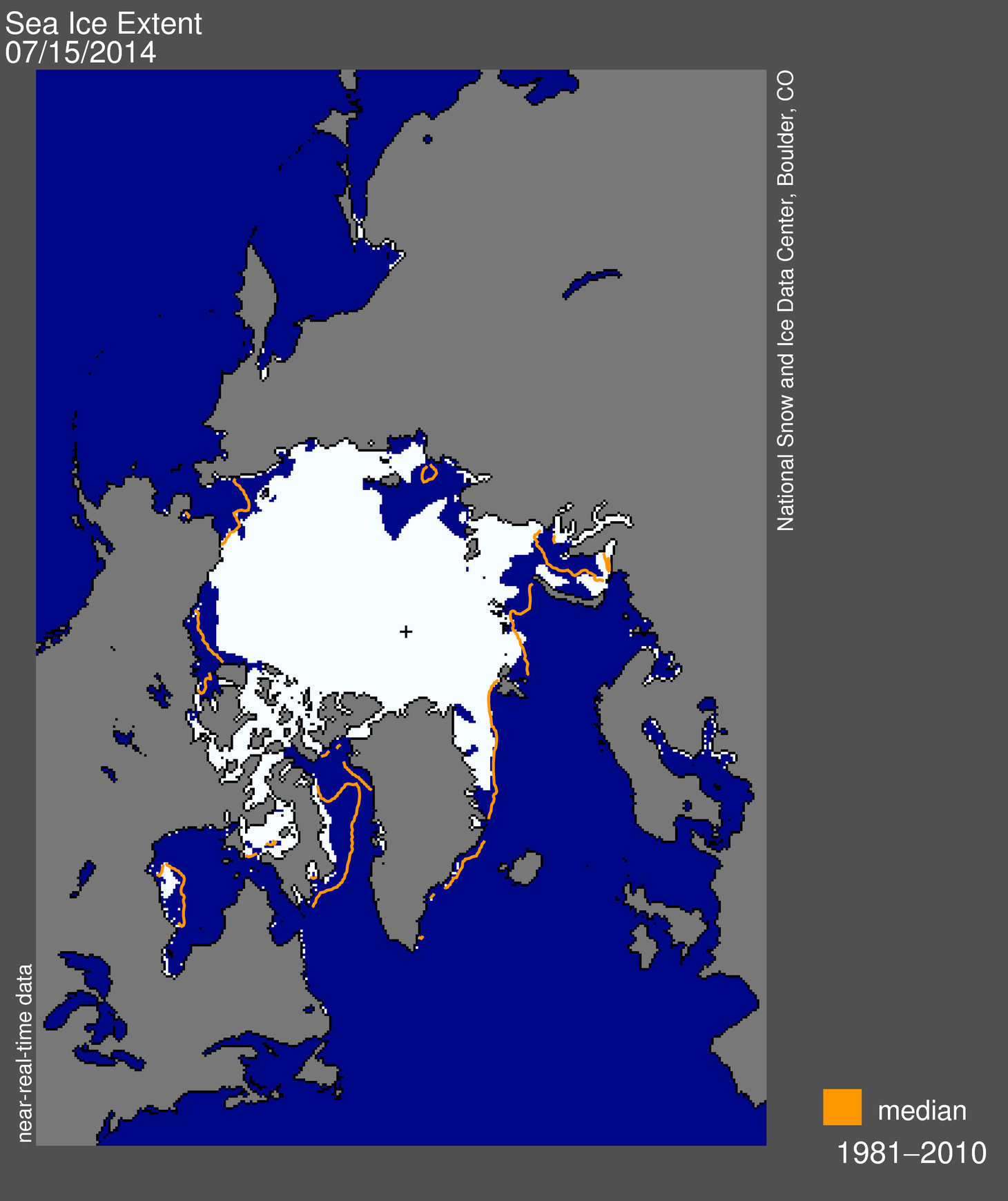
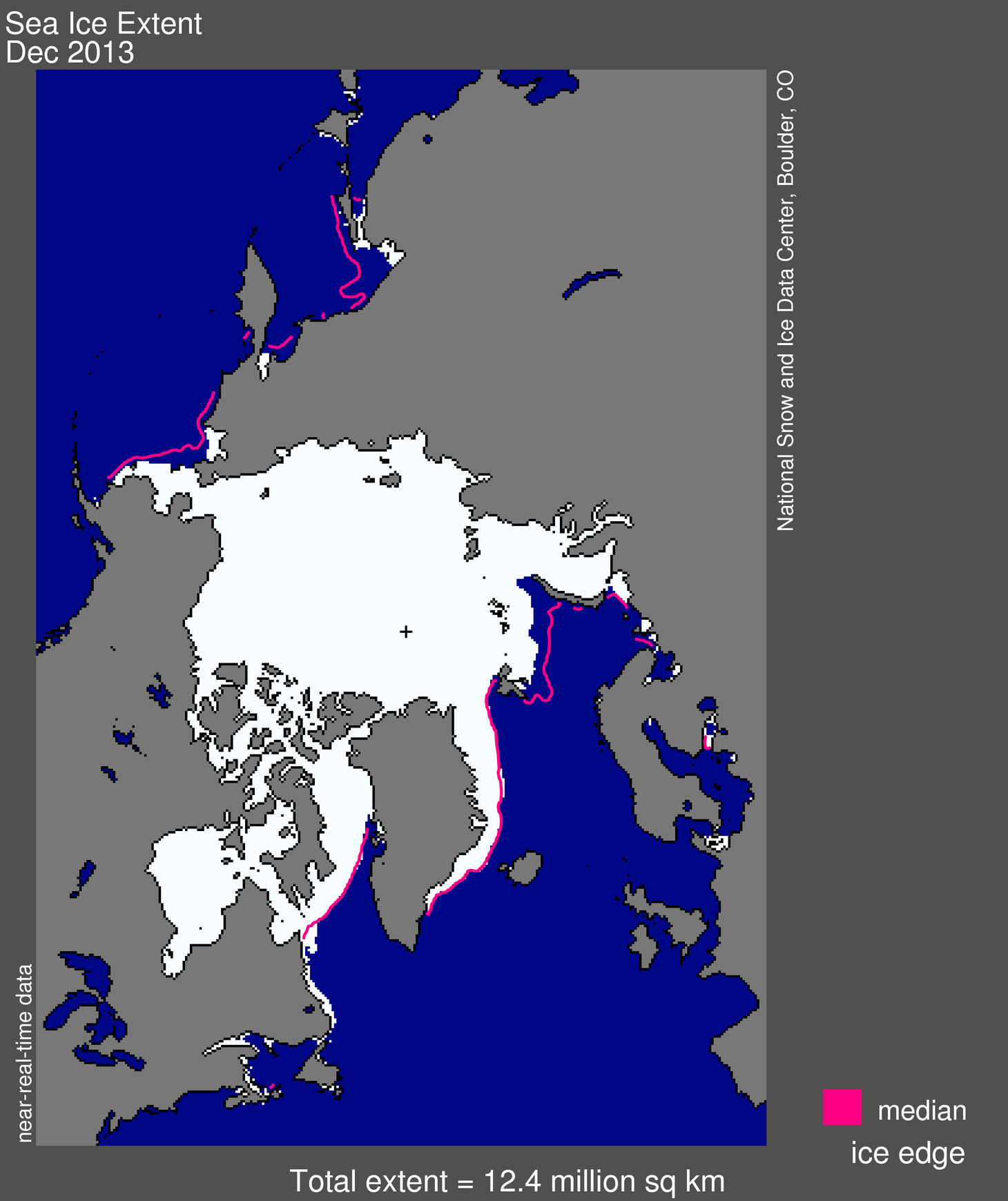
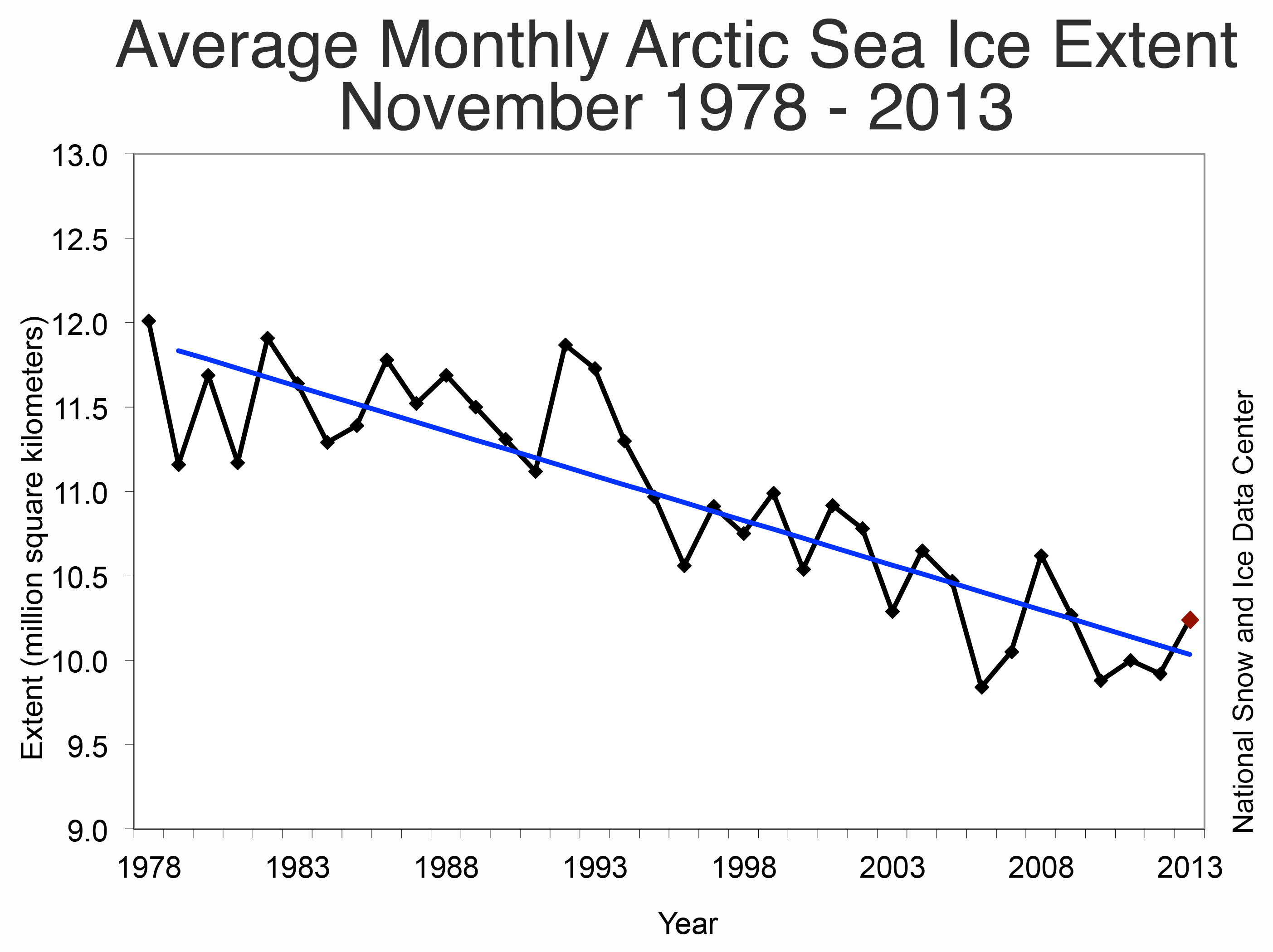
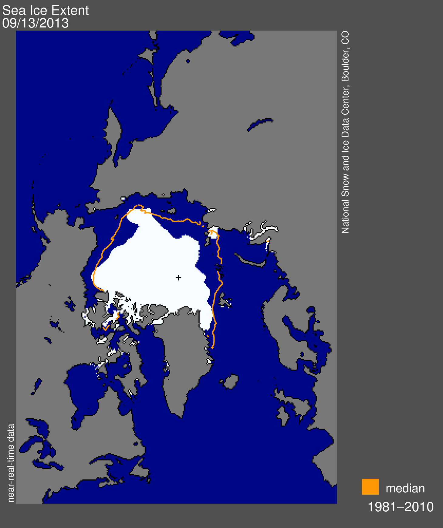
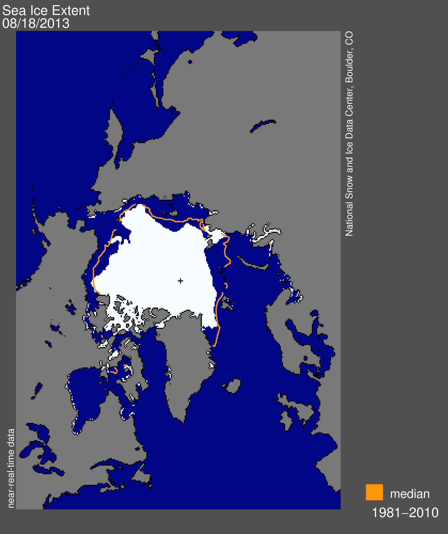
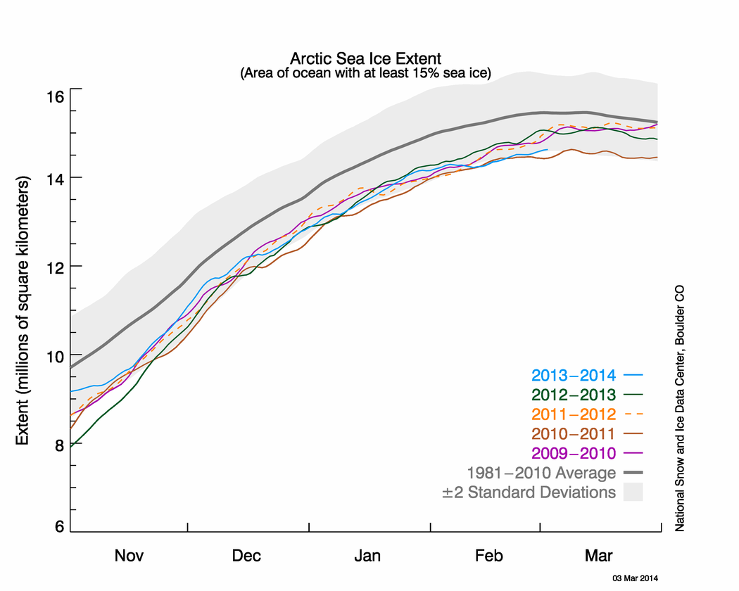
Figure 1. Arctic sea ice extent for July 15, 2014 was 8.33 million square kilometers (3.22 million square miles). The orange line shows the 1981 to 2010 average extent for that month. The black cross indicates the geographic North Pole. Sea Ice Index data. About the data

Credit: National Snow and Ice Data Center
High-resolution image

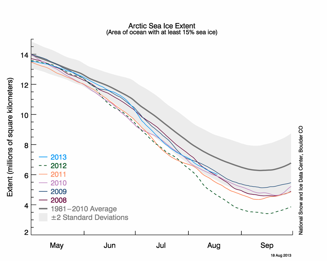
During the second half of June, the rate of sea ice loss in the Arctic was the second fastest in the satellite data record. As a result, by the beginning of July extent fell very close to two standard deviations below the long-term (1981 to 2010) average.

The rate of ice loss for the first half of July averaged 104,000 square kilometers (40,000 square miles) per day, 21% faster than the long-term average for this period.

Ice loss during the first two weeks of July 2014 was dominated by retreat within the Laptev Sea, and within the Kara and Beaufort seas. Open water areas now exist north of 80 degrees North in the Laptev Sea. Ice cover remains fairly extensive in the Beaufort and Kara seas compared to recent summers.

By July 15, ice extent had fallen to within 440,000 square kilometers (170,000 square miles) of that seen in 2012 (the modern satellite-era record minimum) on the same date, and was 1.54 million square kilometers (595,000 square miles) below the 1981 to 2010 average. However, ice concentration remains high within the central Arctic Ocean, particularly compared to 2012.

Conditions in context

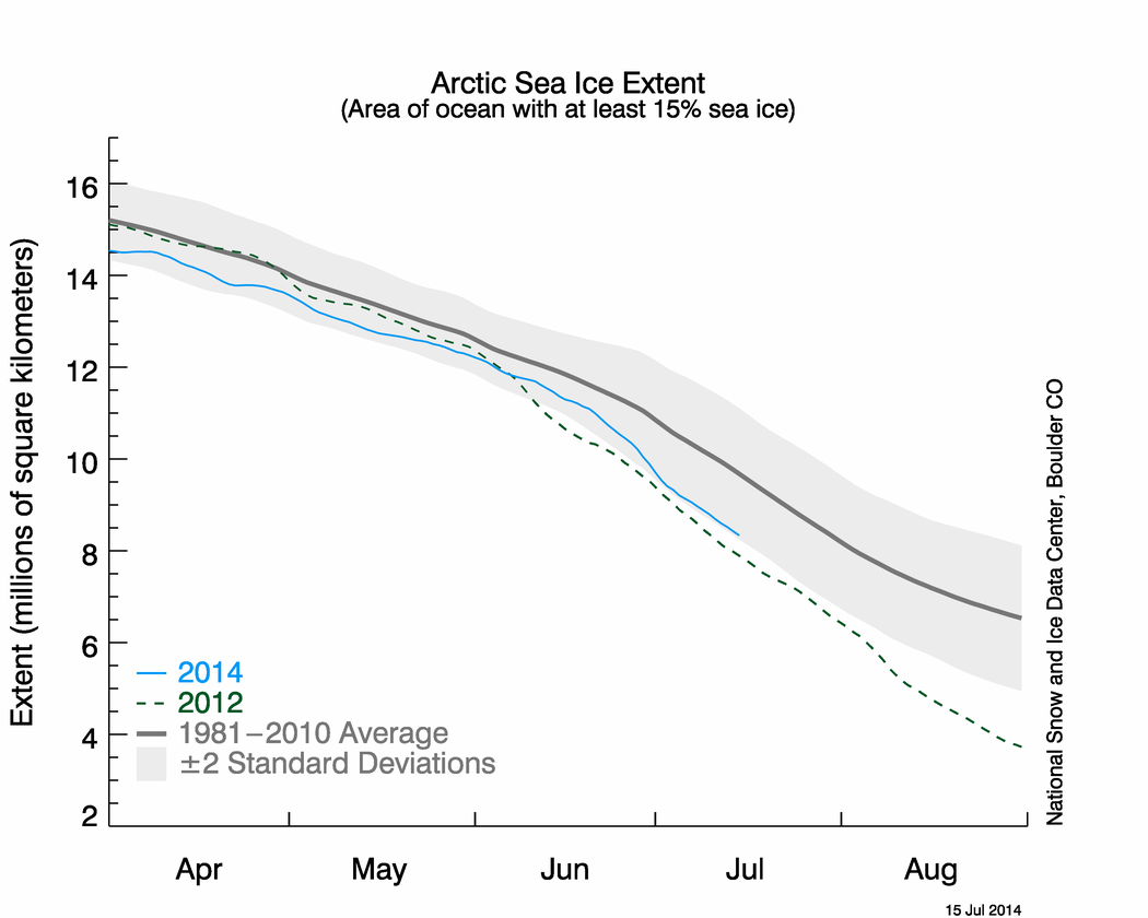
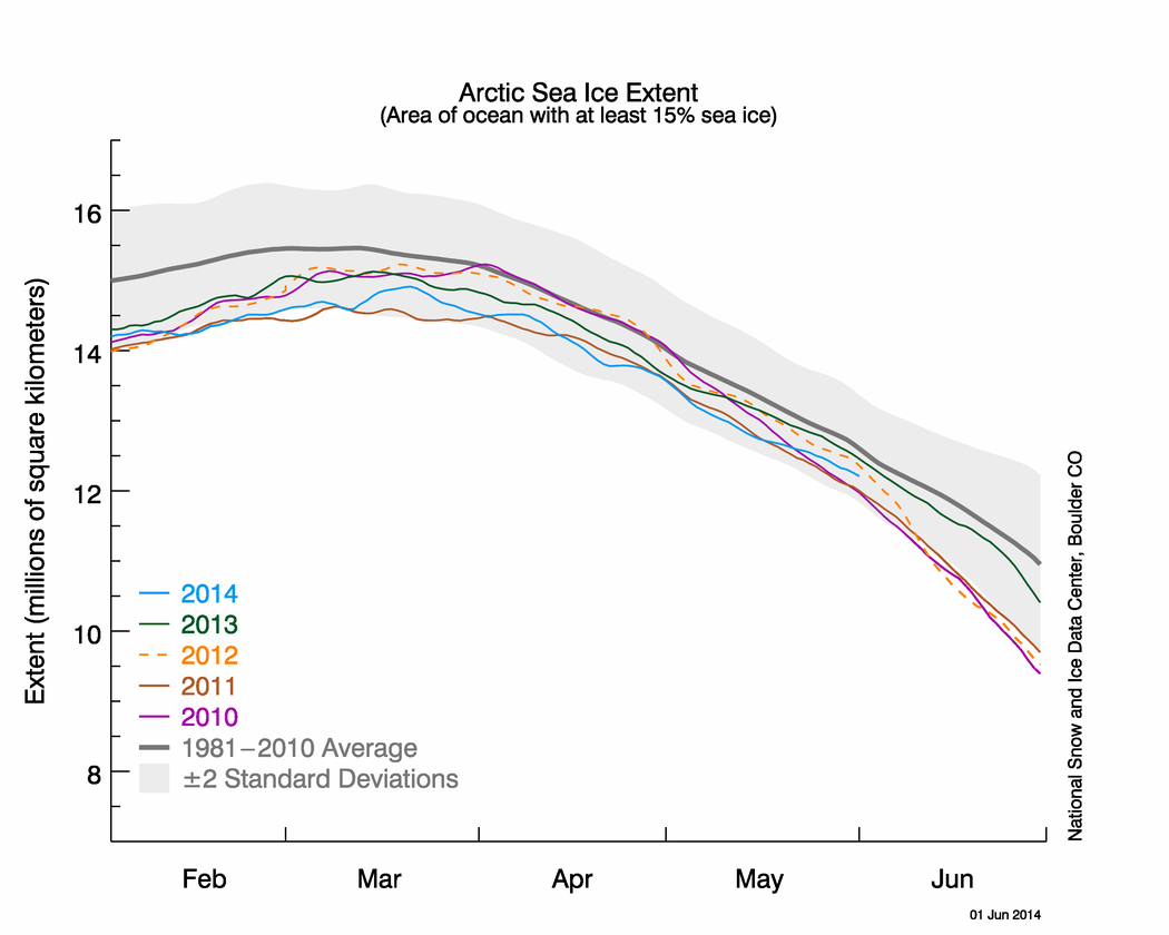
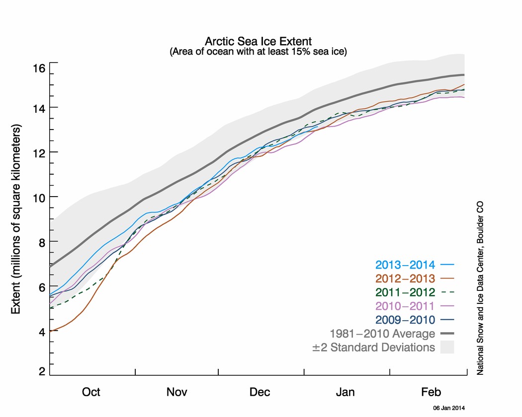
Figure 2. The graph above shows Arctic sea ice extent as of July 15, 2014, along with daily ice extent data for 2012, the record low year. The gray area around the average line shows the two standard deviation range of the data. Sea Ice Index data.

Credit: National Snow and Ice Data Center
High-resolution image

The first half of July 2014 was dominated by anomalously high sea level pressure over the Arctic Ocean and the Barents Sea, coupled with below-average sea level pressure over Iceland. Air temperatures at the 925 millibar level (or about 2,500 feet above the surface) were mostly 1 to 3 degrees Celsius (2 to 5 degrees Fahrenheit) above average over parts of the Arctic Ocean, leading to surface melting. Air temperatures were 1 to 3 degrees Celsius (2 to 5 degrees Fahrenheit) below average in the Kara and Barents seas, where melt has generally been off to a slower start than average this summer. Ice extent remains below average in the Laptev and East Greenland seas and Baffin Bay, and is near average to locally below average in the Beaufort, Chukchi and Kara seas.

Onset of summer melt

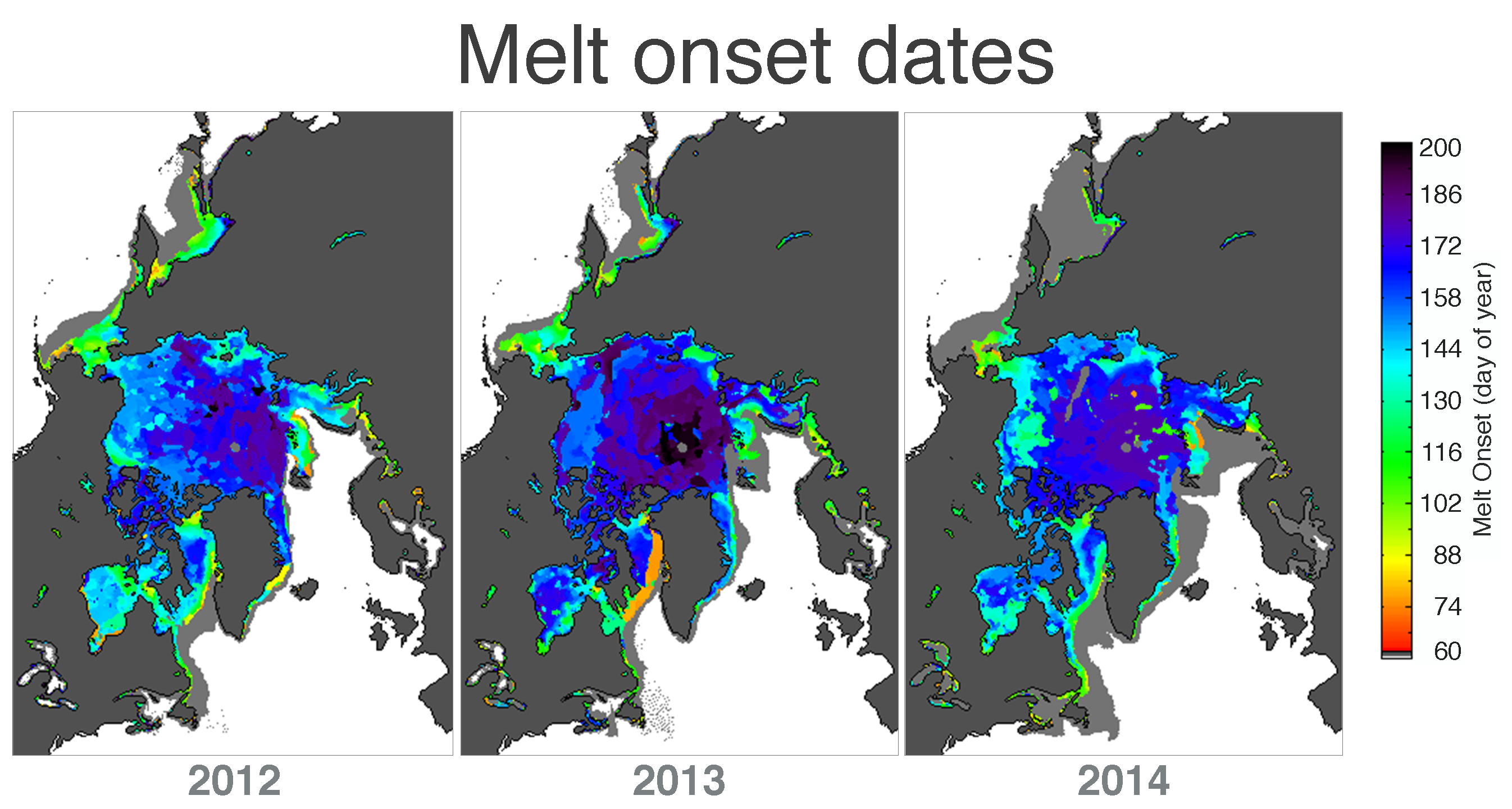
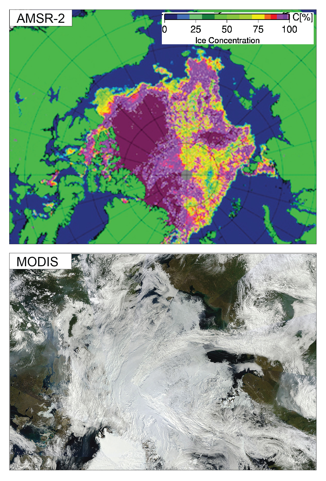
Figure 3a. These images show melt onset dates in the Arctic for 2012, 2013, and 2014 based on the Japan Aerospace Exploration Agency (JAXA) AMSR-2 sensor. Dates are expressed as the day of the year. Areas in light gray are regions where the ice conditions could not permit melt onset detection, or where the melt onset dates are less than day 75. Note that the data for 2014 are preliminary.

Credit: National Snow and Ice Data Center, data provided by J. Miller/T. Markus, NASA Goddard
High-resolution image

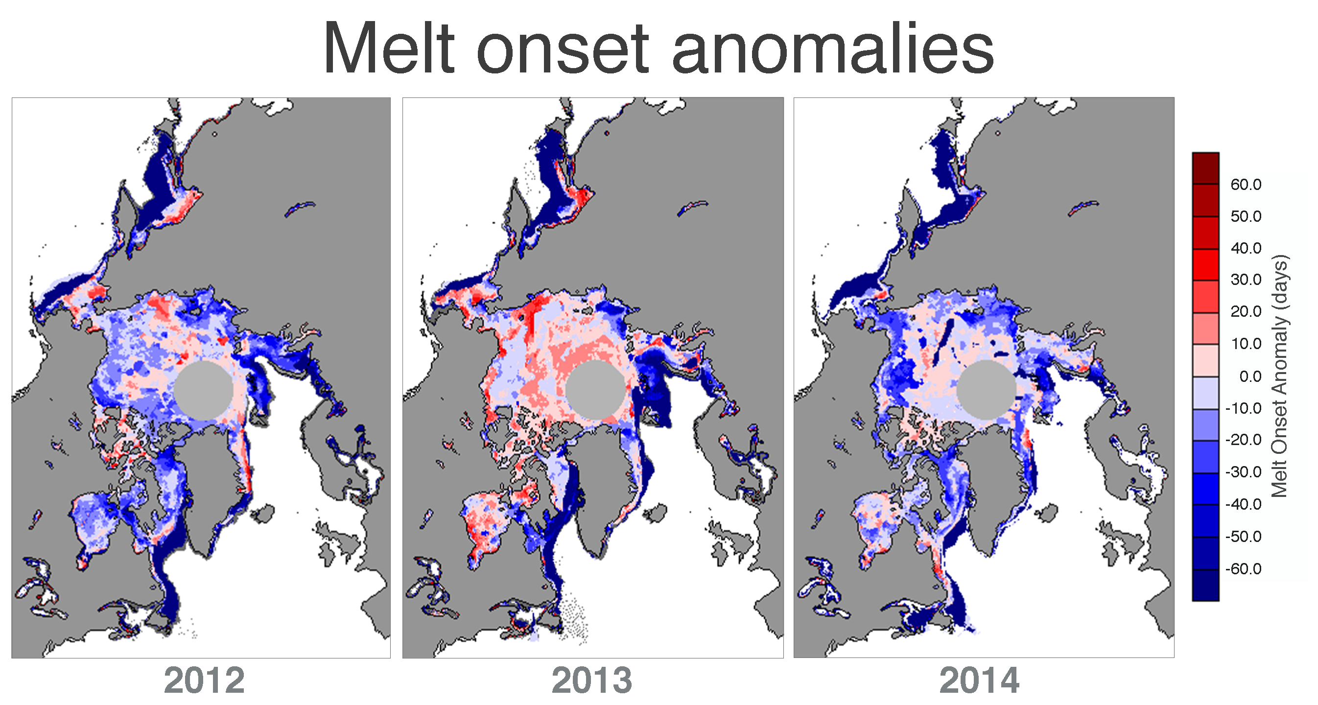
Figure 3b. These images show melt onset anomalies in the Arctic for 2012, 2013, and 2014. Reds indicate areas where melt began later than average and blues indicate melt beginning earlier than average. Since anomalies are computed relative to the 1979 to 2014 long-term average, there is a larger area masked out area around the pole to compensate for the large pole hole during the period of coverage from the Scanning Multichannel Microwave Radiometer (SMMR). Note that the data for 2014 are preliminary.

Credit: National Snow and Ice Data Center, data provided by J. Miller/T. Markus, NASA Goddard
High-resolution image

In general there has been a trend over the satellite data record towards earlier melt onset in the Arctic. Melt usually now begins an average of 7 days earlier than in the late 1970s and early 1980s, or at a rate of about 2 days earlier per decade. However, in regions such as the Kara and Barents seas, melt has begun on average 5 to 7 days per decade earlier, totaling 18 to 25 days earlier since 1979, helping to foster earlier development of open water in those regions.

Despite statistically significant trends towards earlier melt onset, there remains a lot of year-to-year variability. For example, in 2013, melt was slow to start, particularly over the Arctic Ocean, the Laptev and East Siberian seas, Hudson Bay, and the Bering Sea. By contrast, melt onset in 2012 was generally earlier than average over most of the Arctic Ocean, including the Beaufort, Chukchi, Laptev, and Kara seas, as well as Hudson Bay and Baffin Bay, and later than normal in the East Siberian Sea, the Greenland and Bering seas. While melt began earlier than average this summer in the Beaufort, Chukchi, Bering, and Laptev seas, it has been somewhat slower to start in the East Siberian Sea and in the Kara Sea, as well as in large parts of the central Arctic Ocean.

Conditions in Antarctica

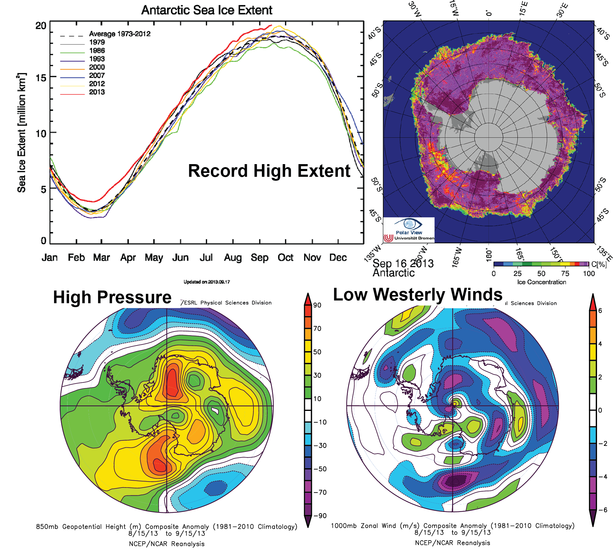
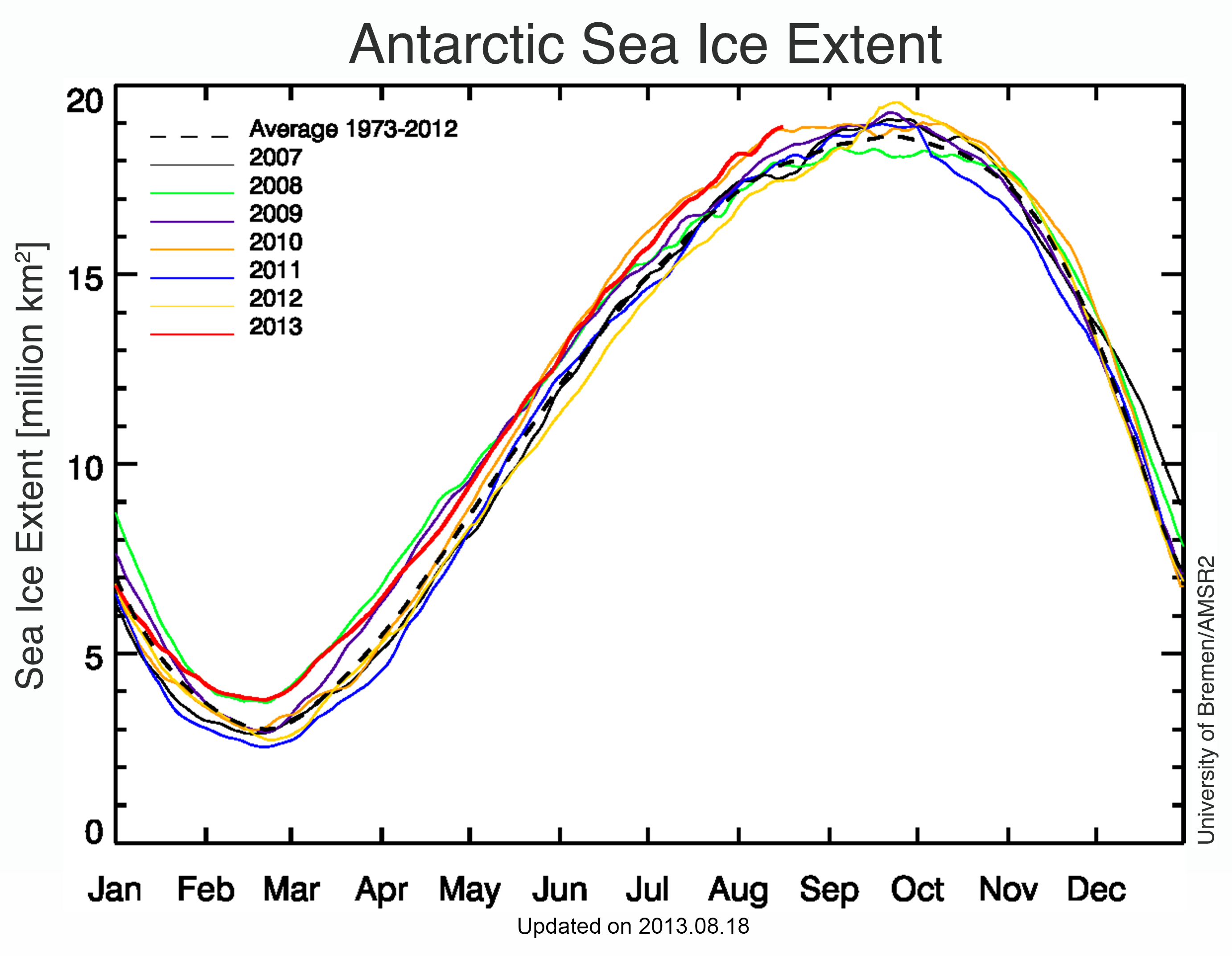
Figure 4. These plots summarize Antarctic sea ice conditions for 2014. The graph at top shows Antarctic sea ice extent as of July 15, 2014, along with daily ice extent data for four previous years. 2014 is shown in blue, 2013 in green, 2012 in orange, 2011 in brown, and 2010 in purple. The 1981 to 2010 average is in dark gray. Sea Ice Index data. The center panel shows the concentration anomaly for June 2014 monthly average extent, indicating three large areas of higher-than-average concentration relative to the 1981 to 2010 average. The lower panel shows an increase of 1.7% per decade in monthly June Antarctic ice extent relative to the 1981 to 2010 average. The four highest June average sea ice extents have been in 2014, 2010, 1979, and 2013. Sea Ice Index data.

Credit: National Snow and Ice Data Center
High-resolution image

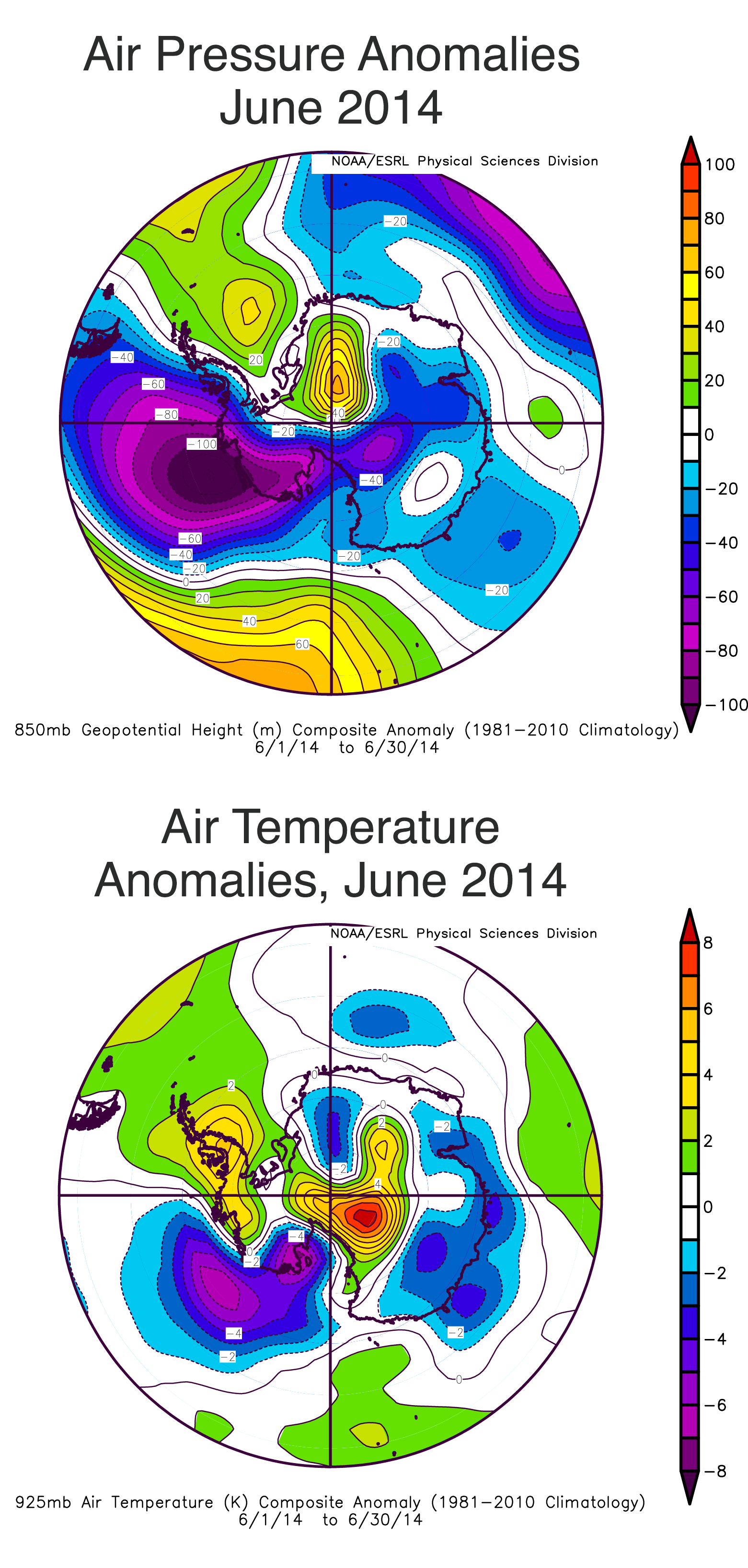
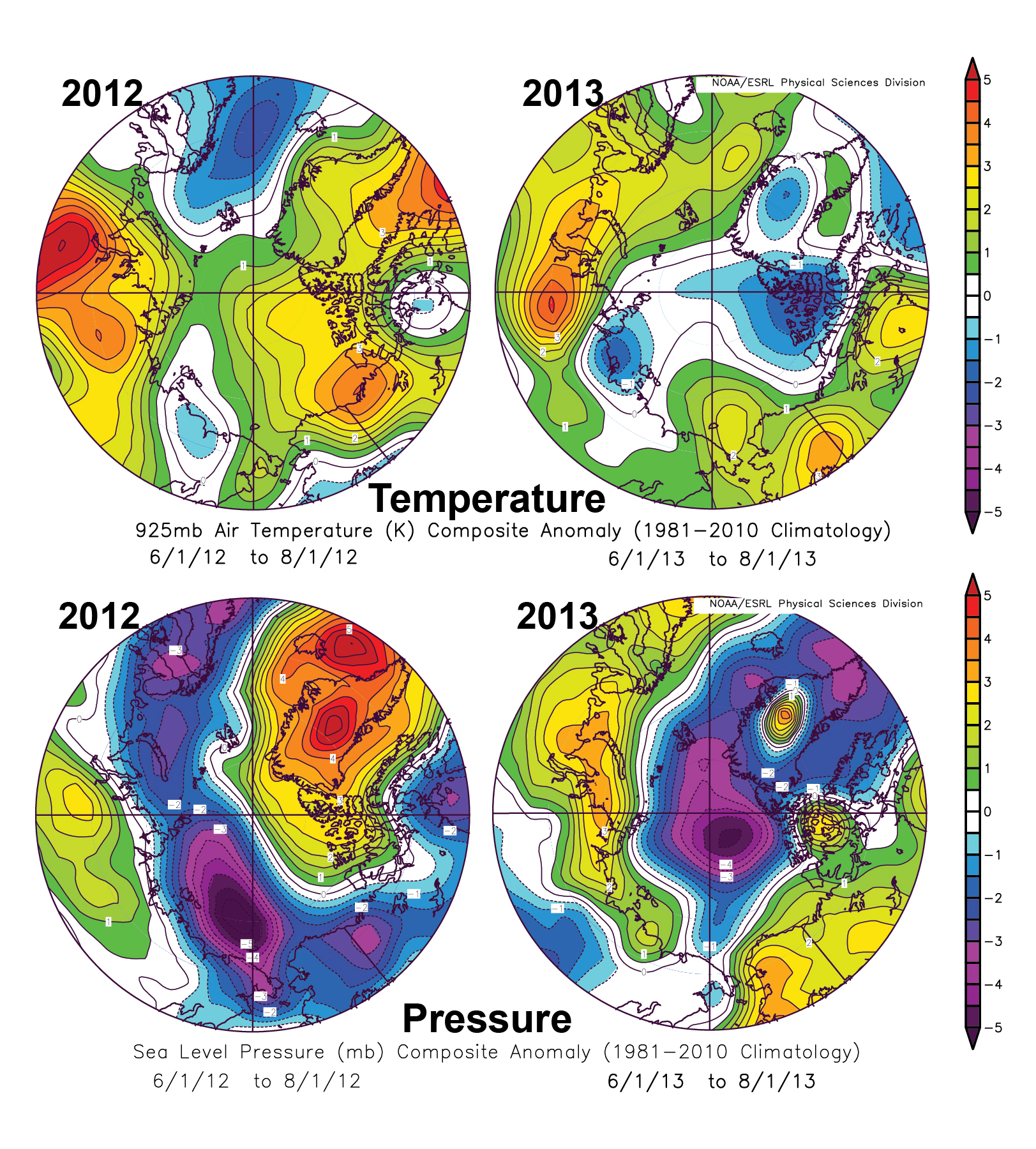
Figure 5. The top image shows the Antarctic sea level air pressure anomaly for June 2014. Blue and purple indicate lower than average pressure; green, yellow, and red indicate higher than average pressure. The bottom plot shows Antarctic air temperature anomalies at the 925 hPa level in degrees Celsius for June 2014. Yellows and reds indicate higher than average temperatures; blues and purples indicate lower than average temperatures.

Credit: NOAA/ESRL Physical Sciences Division
High-resolution image

On July 1, Antarctic sea ice extent was at 16.16 million square kilometers (6.24 million square miles), or 1.37 million square kilometers (529,000 square miles) above the 1981 to 2010 average. More notably, sea ice extent on that date was 760,000 square kilometers (293,000 square miles) higher than the 2013 extent for the same day, and thus is on pace to possibly surpass the record high extent over the period of satellite observations that was recorded last September.

For June, sea ice concentration and extent were higher than average for the Amundsen, Southern Indian Ocean, and far southern Atlantic (Weddell and eastward) sectors. (See Antarctic reference map.) The regions on either side of the Antarctic Peninsula were among the few sections with lower-than-average concentration and lower sea ice extent. Cooler-than-average ocean conditions are present near the ice edge along the Wilkes Land, Amundsen Sea, and Weddell Sea ice edge, which will favor continued expansion of sea ice in these areas.

Weather patterns over Antarctica during June were characterized by a strong low-pressure pattern over the Amundsen Sea, and lower-than-average air temperatures (1 to 6 degrees Celsius, or 2 to 11 degrees Fahrenheit below average) in the same region. Cool conditions (2 to 3 degrees Celsius or 4 to 5 degrees Fahrenheit below average) surrounded most of the coastal areas of the Antarctic, with the exception of the Peninsula region where, as has also been seen in the first two weeks of July, northerly winds brought warmer-than-average conditions and reduced sea ice extent.

Antarctica’s positive trend in sea ice extent

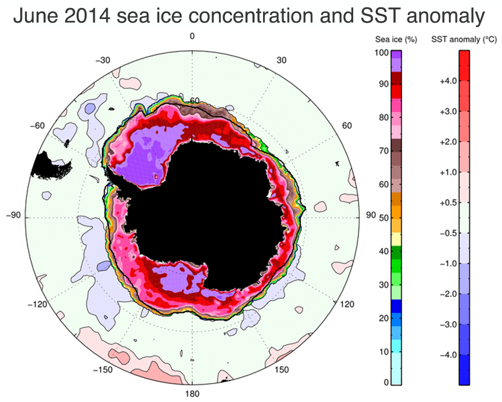
Figure 6. Antarctic sea ice concentration anomaly (deeper colors) and ocean surface temperature anomaly (pastel blue and red) for June 2014. Cool ocean conditions are present around much of the sea ice edge. The average ice edge is shown in black.

Credit: P. Reid, Australia Bureau of Meteorology
High-resolution image

Antarctic sea ice extent also shows a small, long-term upward trend over the period of satellite observations. Antarctica and the Southern Ocean are geographically very different from the Arctic, and are governed by different atmospheric and ocean circulation patterns. Nevertheless, Antarctica has experienced many of the same general signals of Earth’s changing climate as in the Arctic, including general warming, ice sheet loss and faster-flowing glaciers. This makes the small, long-term upward trend in Antarctic sea ice extent rather puzzling. The record sea ice maxima over the past two years (relative to the modern satellite era) have added to the puzzle.

Two recent studies, focused on the back-to-back satellite-era record maxima of 2012 and 2013 (Turner et al., 2013; Reid et al., 2014 in press), point to unusual short-term wind patterns that both fostered ice growth and spread the ice out. In both years, the record-setting extents are related to the size and strength of the Amundsen Sea low pressure area late in the growth season. The more recent study also notes cool ocean water (1 to 2 degrees Celsius or 2 to 4 degrees Fahrenheit below average) persisting near the sea ice edge in the Amundsen-Bellingshausen region in July and August 2013.

Leading ideas regarding the long-term upward trend as assessed over the thirty-five-year satellite record are: (1) persistent changes in wind patterns, resulting from increased westerly winds, which have changed both how much ice is formed and how it is moved around after formation (Holland and Kwok, 2012); and (2) that meltwater from the underside of deep floating ice shelves surrounding the continent (greater than 350 meters, or 1,150 feet thick) has risen to the surface and contributed to a slight freshening of the surface ocean layer (Bintanja et al., 2012). The extra melting results from the changing wind patterns, which act to draw deep warm ocean water inward to the continent to replace surface water and sea ice that is pushed outward and eastward by the stronger westerlies. By thickening, spreading, and stabilizing the polar surface ocean layer (which is comprised of cool, near-freezing water) the increased melt from the ice sheet edges helps sea ice grow around the Antarctic continent.

Early satellite data

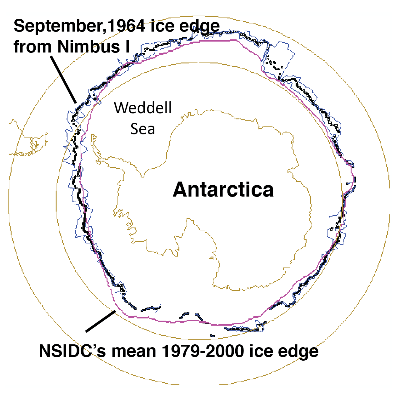
Figure 7. This map of the Antarctic ice edge for September 1964 from the Nimbus I satellite shows greater ice extent than the modern satellite period (1979 to 2014). A similar mapping of the August 1966 sea ice extent showed lower ice extent than modern data have shown for that month. The figure is modified from Gallaher et al., 2014.

Credit: National Snow and Ice Data Center
High-resolution image

Antarctica’s sea ice extent has also been highly variable. For example, austral summer minimum ice extents have varied by as much as 25% over the 1979 to 2014 modern satellite record. The June 1979 extent was the highest for a month by a significant margin. Then in 2002, June sea ice extent was the lowest ever recorded. Nine years later, in June 2011, extent tracked below the 1981 to 2010 average.

This variability is underscored by recent assessments of very early satellite images from the Nimbus program of the late 1960s (Gallaher et al., 2014). Mapping of the September 1964 ice edge (at the austral winter sea ice maximum) indicates that 1964 likely exceeded both the 2012 and 2013 record monthly-average maximums, at 19.7±0.3 million square kilometers (7.60±0.11 million square miles). This was followed in August 1966 by an extent estimated at 15.9±0.3 million kilometers (6.13±0.11 million square miles), considerably smaller than the record low August monthly extent set in 1986. It hence appears that Antarctica’s sea ice variability may be greater than the 35-year modern satellite record would indicate, and that the current growth trend, while important, is not yet reaching unprecedented levels seen within the past century.

Further reading

Bintanja, R., G. J. Van Oldenborgh, S. S. Drijfhout, B. Wouters, and C. A. Katsman. 2013. Important role for ocean warming and increased ice-shelf melt in Antarctic sea-ice expansion, Nature Geoscience, 6, 376–379, doi:10.1038/ngeo1767.

Gallaher, D., G. G. Campbell, and W. N. Meier. 2014. Anomalous variability in Antarctic sea ice extents during the 1960s with the use of Nimbus data. IEEE Journal of Selected Topics in Applied Earth Observations and Remote Sensing, 7(3), 881-887, doi:10.1109/JSTARS.2013.2264391.

Holland, P., and R. Kwok. 2012. Wind-driven trends in Antarctic sea-ice drift. Nature Geoscience, 5(12), 872-875, doi:10.1038/ngeo1627.

Reid, P., S. Stammerjohn, R. Massom, T. Scambos, and J. Leiser. 2014 in press. The record 2013 Southern Hemisphere sea-ice extent maximum. Annals of Glaciology, in press, 64(69).

Turner J., J. S. Hosking, T. Phillips, and G. J. Marshall. 2013. Temporal and spatial evolution of the Antarctic sea ice prior to the September 2012 record maximum extent. Geophysical Research Letters, 40, 5894–5898, doi:10.1002/2013GL058371.

Arctic sea ice extent declined at a typical rate through May, but extent remained below average for the period of satellite observations. While Antarctic sea ice extent increased at a near average rate, extent was at a record high, and above average in nearly every Antarctic sea ice sector.

Overview of conditions

Figure 1. Arctic sea ice extent for May 2014 was 12.78 million square kilometers (4.93 million square miles). The magenta line shows the 1981 to 2010 median extent for that month. The black cross indicates the geographic North Pole. Sea Ice Index data. About the data

Credit: National Snow and Ice Data Center
High-resolution image

Arctic sea ice extent for May averaged 12.78 million square kilometers (4.93 million square miles). This is 610,000 square kilometers (235,500 square miles) below the 1981 to 2010 average for the month. May 2014 is now the third lowest May extent in the satellite record.

Ice extent was lower than average in the Barents and Bering seas. While not visible in the monthly average extent plot, the evolution of the sea ice through the month of May is characterized by the opening of several polynyas along the coast of Siberia, northern Baffin Bay, and along the coast of Hudson Bay. Nevertheless, satellites detected high sea ice concentrations over the Arctic as a whole. This contrasts with 2006, 2007, and 2012 when broad areas of low-concentration ice were observed.

As the melt season is underway in the Arctic, freeze up is in progress in the Antarctic. Sea ice extent for May averaged 12.03 million square kilometers (4.64 million square miles). This is 1.24 million square kilometers (478,800 square miles) above the 1981 to 2010 average for the month. Antarctic sea ice for May 2014 currently ranks as the highest May extent in the satellite record.

Conditions in context

Figure 2. The graph above shows Arctic sea ice extent as of June 1, 2014, along with daily ice extent data for four previous years. 2014 is shown in blue, 2013 in green, 2012 in orange, 2011 in brown, and 2010 in purple. The 1981 to 2010 average is in dark gray. Sea Ice Index data.

Credit: National Snow and Ice Data Center
High-resolution image

May ice extent for the Arctic declined at a fairly steady rate. Sea ice retreated most rapidly in the northern Bering and southern Chukchi seas, and in the Barents Sea where a small area south of the Franz Josef Land archipelago opened late in the month. Weather was dominated by lower-than-average sea level pressure over the Central Arctic Ocean, and higher-than-average pressure over the southern Bering Sea, Alaska, and Canada. This brought about lower-than-average temperatures in the North Greenland Sea and extended toward the poles, as assessed at the 925 hPa level (roughly 3,000 feet). In contrast, warm conditions prevailed over northern Hudson Bay and southern Alaska (2 to 5 degrees Celsius or 4 to 9 degrees Fahrenheit above the 1981 to 2010 average) and the Kara and Laptev seas (1 to 2 degrees Celsius or 2 to 4 degrees Fahrenheit above the 1981 to 2010 average).

May 2014 compared to previous years

Figure 3. Monthly May ice extent for 1979 to 2014 shows a trend of -2.3% per decade relative to the 1981 to 2010 average.

Credit: National Snow and Ice Data Center
High-resolution image

Arctic sea ice extent dropped at a rate of –44,300 square kilometers (–17,100 square miles) per day, close to the average rate of –45,700 square kilometers (–17,700 square miles) per day. The monthly trend for May is now –2.3% per decade relative to the 1981 to 2010 average.

In the Antarctic, sea ice extent increased at a rate of 108,500 square kilometers (41,900 square miles) per day, very close to the average rate of 108,400 square kilometers (41,850 square miles) per day. For Antarctica, the linear rate of increase for May ice extent is 2.6% per decade relative to the 1981 to 2010 average.

Northern Hemisphere snow cover retreats rapidly

Figure 4a. This snow cover anomaly map shows the difference between snow cover for May 2014, compared with average snow cover for May from 1981 to 2010. Areas in orange and red indicate lower than usual snow cover, while regions in blue had more snow than normal.

Credit: National Snow and Ice Data Center, courtesy Rutgers University Global Snow Lab
High-resolution image

Figure 4b. This graphs shows snow cover extent anomalies in the Northern Hemisphere for May from 1967 to 2014. The anomaly is relative to the 1981 to 2010 average.

Credit: National Snow and Ice Data Center, courtesy Rutgers University Global Snow Lab
High-resolution image

After a greater-than-average snow extent in February, snow extent over the Northern Hemisphere shrank rapidly in March, April and May. The Rutgers University Global Snow Lab measured the lowest April snow extent in Eurasia in the 48-year data record. (Erratum: In an earlier version of this post, we mistakenly said that the record low April snow cover was observed in the Northern Hemisphere. We apologize for the error.) In May, snow rapidly retreated in the central Canadian Provinces in North America, and Central Asia (Kazakhstan and northwestern China), where extensive areas had above-average snow cover in February.

Snow cover in central Europe and the desert southwest of the United States were persistently below average throughout the winter and spring of 2013 to 2014. In the United States, this underscores the severe drought in the far southwest and Sierra Nevada. The rapid late spring loss in the Northern Hemisphere continues a decade-long trend toward very low snow cover early in the Arctic sea ice melt season. This resulted in warmer air over darker snow-free areas, which leads to warm air advection over the sea ice

in regions where the snow cover is anomalously low, and dry conditions in the northern boreal forests. These conditions cause increased wildfire activity and soot deposition on the sea ice and the Greenland Ice Sheet surface. High concentrations of soot on the Greenland snow pack and sea ice can contribute to ice retreat and melt.

New Arctic sea ice thickness quick look products from IceBridge, ESA CryoSat-2

Figure 5a. Data from NASA Operation IceBridge flights over the Arctic Ocean during March and April 2014.

Credit: National Snow and Ice Data Center/NASA Operation IceBridge courtesy Nathan Kurtz
High-resolution image

Figure 5b. This figure shows Arctic sea ice thickness for March 2014 using data from the European Space Agency’s CryoSat-2 satellite.

Credit: National Snow and Ice Data Center/NASA Operation IceBridge courtesy Nathan Kurtz
High-resolution image

The NASA IceBridge mission is an airborne campaign to augment and validate satellite measurements of sea ice and ice sheets. This spring, the NASA IceBridge program set a new record of 46 science flights, covering almost 150,000 kilometers (93,200 miles) of flight tracks from March 12, 2014 to April 3, 2014. This included flights over the western Arctic Ocean and north of Greenland to map sea ice thickness and snow depth. NSIDC has published the 2014 quick look product, in addition to a new ESA CryoSat-2 derived sea ice thickness product. Thickness estimates from both products suggest large areas within the western Beaufort Sea that are 1 to 1.5 meters (3 to 5 feet) thick. The tongue of second-year ice that extends up toward the East Siberian Sea is considerably thicker, at 2 to 3 meters (7 to 10 feet) thick. In the eastern Arctic, the ice is predominantly first-year ice, and between 1 and 1.5 meters (3 to 5 feet) thick. The thickest ice is found north of Greenland and near the pole, ranging from 3.5 to 5 meters (11 to 16 feet) thick. The timely release of thickness data from IceBridge and ESA CryoSat-2 provide a valuable resource for seasonal forecasting because they provide an estimate of the ice thickness distribution in the Arctic at the beginning of the melt season.

Forecasting needs for Arctic weather and sea ice

The National Oceanic and Atmospheric Administration (NOAA) and the U.S. Navy share a pressing need for better short-term sea ice and weather forecasts to meet their operational responsibilities. With this as a driver, the NOAA Earth Systems Research Laboratory (ESRL) hosted a workshop on Predicting Arctic Weather and Climate, and Related Impacts: Status and Requirements for Progress. The meeting was held on May 13 to 15 in Boulder, Colorado. Participants from the Office of Naval Research and the oceanographer of the Navy’s office outlined their perspective on needs for operational predictions. National Weather Service participants spoke about operational forecasting, while scientists under NOAA’s research arm along with academic scientists gave talks tailored to answering questions from forecasters. The Navy/NOAA/Coast Guard National Ice Center participated as a prime customer for better forecasting capability out of the research community. Operational needs are greatest for forecasts six to eight weeks out, where better availability of data to initialize coupled atmospheric/ocean models offers promise for improvement. Seasonal forecasts of ice melt can be improved with better ice thickness initialization fields. The predictability of the timing of freeze-up at the end of the season appears to depend upon improved sea surface temperature fields.

The NOAA Arctic Action Plan and the U.S. Navy’s Arctic Roadmap give a high-level view of how these agencies are addressing change in the Arctic.

Reference

Kurtz, N. T., Galin, N., and Studinger, M. 2014. An improved CryoSat-2 sea ice freeboard and thickness retrieval algorithm through the use of waveform fitting, The Cryosphere Discuss., 8, 721-768, doi:10.5194/tcd-8-721-2014.

Overview of conditions

Figure 1. Arctic sea ice extent for March 2014 was 14.80 million square kilometers (5.70 million square miles). The magenta line shows the 1981 to 2010 median extent for that month. The black cross indicates the geographic North Pole. Sea Ice Index data. About the data

Credit: National Snow and Ice Data Center
High-resolution image

Arctic sea ice extent for March 2014 averaged 14.80 million square kilometers (5.70 million square miles). This is 730,000 square kilometers (282,000 square miles) below the 1981 to 2010 average extent, and 330,000 square kilometers (127,000 square miles) above the record March monthly low, which happened in 2006. Extent remains slightly below average in the Barents Sea and the Sea of Okhotsk, but is at near-average levels elsewhere. Extent hovered around two standard deviations below the long-term average through February and early March. The middle of March by contrast saw a period of fairly rapid expansion, temporarily bringing extent to within about one standard deviation of the long-term average.

Conditions in context

Figure 2. The graph above shows Arctic sea ice extent as of April 1, 2014, along with daily ice extent data for four previous years. 2013 to 2014 is shown in blue, 2012 to 2013 in green, 2011 to 2012 in orange, 2010 to 2011 in brown, and 2009 to 2010 in purple. The 1981 to 2010 average is in dark gray. Sea Ice Index data.

Credit: National Snow and Ice Data Center
High-resolution image

In the Arctic, the maximum extent for the year is reached on average around March 9. However, the timing varies considerably from year to year. This winter the ice cover continued to expand until March 21, reaching 14.91 million square kilometers (5.76 million square miles), making it both the fifth lowest maximum and the fifth latest timing of the maximum since 1979. The latest timing of the maximum extent was on March 31, 2010 and the lowest maximum extent occurred in 2011 (14.63 million square kilometers or 5.65 million square miles).

The late-season surge in extent came as the Arctic Oscillation turned strongly positive the second week of March. This was associated with unusually low sea level pressure in the eastern Arctic and the northern North Atlantic. The pattern of surface winds helped to spread out the ice pack in the Barents Sea where the ice cover had been anomalously low all winter. Northeasterly winds also helped push the ice pack southwards in the Bering Sea, another site of persistently low extent earlier in the 2013 to 2014 Arctic winter. Air temperatures however remained unusually high throughout the Arctic during the second half of March, at 2 to 6 degrees Celsius (4 to 11 degrees Fahrenheit) above the 1981 to 2010 average.

March 2014 compared to previous years

Figure 3. Monthly March ice extent for 1979 to 2014 shows a decline of 2.6% per decade relative to the 1981 to 2010 average.

Credit: National Snow and Ice Data Center
High-resolution image

Average ice extent for March 2014 was the fifth lowest for the month in the satellite record. Through 2014, the linear rate of decline for March ice extent is 2.6% per decade relative to the 1981 to 2010 average.

An increase in multiyear ice

Figure 4. Imagery from the European Advanced Scatterometer (ASCAT) show the distribution of multiyear ice compared to first year ice for March 28, 2013 (yellow line) and March 2, 2014 (blue line).

Credit: Advanced Scatterometer imagery courtesy NOAA NESDIS, analysis courtesy T. Wohlleben, Canadian Ice Service
High-resolution image

The extent of multiyear ice within the Arctic Ocean is distinctly greater than it was at the beginning of last winter. During the summer of 2013, a larger fraction of first-year ice survived compared to recent years. This ice has now become second-year ice. Additionally, the predominant recirculation of the multiyear ice pack within the Beaufort Gyre this winter and a reduced transport of multiyear ice through Fram Strait maintained the multiyear ice extent throughout the winter.

In Figure 4, Advanced Scatterometer (ASCAT) imagery reveals the distribution of multiyear ice compared to first year ice for March 28, 2013 (yellow line) and March 2, 2014 (blue line). The ASCAT sensor measures the radar–frequency reflection brightness of the sea ice at a few kilometers resolution. Sea ice radar reflectivity is sensitive to the roughness of the ice and the presence of saltwater droplets within newer ice (and, later in the season, the presence of surface melt). Thus older and more deformed multiyear ice appears white or light grey (more reflection), whereas younger, first-year ice looks dark grey and/or black.

Ice age tracking confirms large increase in multiyear ice

Figure 5. The map at top shows the ages of ice in the Arctic at the beginning of March 2014; the bottom graph shows how the percentage of ice in each age group has changed from 1983 to 2014 .

Credit: NSIDC, Courtesy M. Tschudi, University of Colorado
High-resolution image

Satellite data on ice age reveal that multiyear ice within the Arctic basin increased from 2.25 to 3.17 million square kilometers (869,000 to 1,220,000 square miles) between the end of February in 2013 and 2014. This winter the multiyear ice makes up 43% of the icepack compared to only 30% in 2013. While this is a large increase, and may portend a more extensive September ice cover this year compared to last year, the fraction of the Arctic Ocean consisting of multiyear ice remains less than that at the beginning of the 2007 melt season (46%) when a large amount of the multiyear ice melted. The percentage of the Arctic Ocean consisting of ice at least five years or older remains at only 7%, half of what it was in February 2007. Moreover, a large area of the multiyear ice has drifted to the southern Beaufort Sea and East Siberian Sea (north of Alaska and the Lena River delta), where warm conditions are likely to exist later in the year.

Summer ice extent remains hard to predict

Figure 6. Median (red) and interquartile range (gray shading) of sea ice predictions submitted to the July SEARCH SIO each year compared with September mean sea ice extent (green).

Credit: Stroeve et al.
High-resolution image

There is a growing need for reliable sea ice predictions. An effort to gather and summarize seasonal sea ice predictions made by researchers and prediction centers began in 2008. The project, known as the SEARCH Sea Ice Outlook, has collected more than 300 predictions of summer month ice extent. A new study published in Geophysical Research Letters by researchers at NSIDC, University of New Hampshire, and University of Washington reveal a large range in predictive skill. The study found that forecasts are quite accurate when sea ice conditions are close to the downward trend that has been observed in Arctic sea ice for the last 30 years. However, forecasts are not so accurate when sea ice conditions are unusually higher or lower compared to this trend. Results from the study also suggest that while ice conditions during the previous winter are an important predictor (such as the fraction of first-year versus multiyear ice), summer weather patterns also have a large impact on the amount of ice that will be left at the end of summer.

Satellite Observations of Arctic Change

NSIDC now offers a new Web site, Satellite Observations of Arctic Change (SOAC)  with interactive maps of the Arctic based on NASA satellite and related data. The site allows you to explore how conditions in the Arctic have changed over time. Data sets include air temperature, water vapor, sea ice, snow cover, NDVI, soil freezing, and exposed snow and ice. Time periods vary by data set, but range from 1979 to 2013. You can animate a time series, zoom in or out, and view a bar graph of anomalies over time. Links to the source data and documentation are also included. Additional pages provide brief scientific discussion, and overviews of the scientific importance of these data. SOAC was developed with support from NASA Earth Sciences.

Reference

Stroeve, J., L. Hamilton, C. M. Bitz, and E. Blanchard-Wrigglesworth. 2014. Predicting September Sea Ice: Ensemble Skill of the SEARCH Sea Ice Outlook 2008–2013. Geophysical Research Letters, Accepted, doi: 10.1002/2014GL059388.

Correction

In the caption for Figure 5, we described the map as showing the ages of ice in the Arctic at the end of March. A reader pointed out that this image was for the beginning of March, which is correct. We regret the error and corrected the caption on April 2, 2014 at 1:25 p.m.

While the eastern half of the United States has dealt with a cold and snowy winter, temperatures in the Arctic have been distinctly higher than average. The warm conditions have led to a slower than average expansion of the winter ice cover. Less ice also contributes to higher air temperatures by allowing transfer of heat from the relatively warmer ocean. The annual maximum in sea ice extent is expected to occur sometime this month.

Overview of conditions

Figure 1. Arctic sea ice extent for February 2014 was 14.44 million square kilometers (5.58 million square miles). The orange line shows the 1981 to 2010 median extent for that month. The black cross indicates the geographic North Pole. Sea Ice Index data. About the data

Credit: National Snow and Ice Data Center
High-resolution image

Arctic sea ice extent in February 2014 averaged 14.44 million square kilometers (5.58 million square miles). This is the fourth lowest February ice extent in the satellite data record, and is 910,000 square kilometers (350,000 square miles) below the 1981 to 2010 average. The lowest February in the satellite record occurred in 2005.

Overall, sea ice grew slowly through the month of February. There were periods of declining ice, likely related to changes in ice motion. Bering Sea ice cover has been below average throughout winter, in contrast to the last several winters. Ice extent also remains below average in the Barents Sea and the Sea of Okhotsk, helping to keep the Arctic ice extent two standard deviations below the 1981 to 2010 average.

Conditions in context

Figure 2. The graph above shows Arctic sea ice extent as of March 3, 2014, along with daily ice extent data for five previous years. 2013-2014 is shown in blue, 2012-2013 in green, 2011-2012 in orange, 2010-2011 in brown, and 2009-2010 in purple. The 1981 to 2010 average is in dark gray. Sea Ice Index data.

Credit: National Snow and Ice Data Center
High-resolution image

Ice extent increased at an average daily rate of 14,900 square kilometers (5,750 square miles) per day through the month of February. This is about 25% slower than the 1981 to 2010 February average rate of 20,300 square kilometers (7,840 square miles) per day. As the maximum extent approaches, the daily rate of ice extent growth is expected to slow.

While the eastern half of the U.S. has suffered through a cold and sometimes snowy winter, conditions in the Arctic have been warmer than average. The Arctic in winter is still a very cold place and temperatures at the 925 mb level in the central Arctic averaged -25 to -15 degrees Celsius (-13 to 5 degrees Fahrenheit); however, this was 4 to 8 degrees Celsius (7 to 14 degrees Fahrenheit) above average for the month. The Arctic Oscillation settled into a near-neutral mode for February after swinging from a strong positive mode in December to a negative mode in January.

February 2014 compared to previous years

Figure 3. Monthly February ice extent for 1979 to 2014 shows a decline of -3.0% per decade per decade relative to the 1981 to 2010 average.

Credit: National Snow and Ice Data Center
High-resolution image

The sea ice extent trend through February 2014 is -3.0% per decade relative to the 1981 to 2010 average, a rate of -46,100 square kilometers (-17,800 square miles) per year. Unlike the summer, where ice loss has accelerated over the past decade, winter month trends have been fairly consistent.

The two Bs of the Arctic: Barents and Bering

Figure 4a. Barents Sea ice extent during February from the NSIDC Multisensor Analyzed Sea Ice Extent (MASIE) for the years 2010 through 2014. MASIE is produced daily by the U.S. National Ice Center based on human analysis of a variety of available satellite imagery.

Credit: National Snow and Ice Data Center and the National Ice Center
High-resolution image

Figure 4b. Bering Sea ice extent during February from the NSIDC Multisensor Analyzed Sea Ice Extent (MASIE) for the years 2010 through 2014. MASIE is produced daily by the U.S. National Ice Center based on human analysis of a variety of available satellite imagery.

Credit: National Snow and Ice Data Center and the National Ice Center
High-resolution image

The Barents Sea has experienced consistently low extents, particularly in winter, and this year has been no different. While the Barents and Kara seas normally have close to 2 million square kilometers (772,000 square miles) of ice in February, recent years have seen 500,000 square kilometers (193,000 square miles) of ice extent or lower. This year, the Kara Sea is near average, but the Barents Sea remains low (Figure 4a). Unlike other regions in the Arctic, longer records of Barents Sea ice extent exist from records of fishing, whaling, and other activities. A recent paper (Miles et al., 2013) examined these records, along with paleoproxy data, to examine extent over the past four hundred years. They found a 60- to 90-year cycle in Barents and Greenland seas ice extent related to the Atlantic Multidecadal Oscillation (AMO); the AMO is a basin-wide cycle of sea surface temperature variability similar to the El Niño and La Niña cycles in the Pacific, but varying over much longer periods. This research shows that in addition to the warming trend in the Arctic, some sea ice regions are likely also responding to natural climate variability.

In contrast to the Barents, the Bering Sea ice has had higher than average extent in recent years. However this year is different; Bering Sea ice extent has been below average through much of the winter. During mid-February, extent increased to a higher level, as seen in Multisensor Analyzed Sea Ice Extent (MASIE) data (Figure 4b), before a slight decline at the end of the month. This is in contrast with recent years in the Bering that have seen very high extents, even record levels .

The Bering Sea consists exclusively of seasonal ice with a large marginal ice zone where new, thin ice dominates. Sea ice in this region is quite sensitive to changes in temperatures and, particularly, winds. Cold winds from the north advect ice southward and aid new ice growth. Warm winds from the south impede ice growth and push the ice northward, reducing extent in the region. Recent winters have been characterized by predominantly north winds. This year represents a change with more zonal, east to west, winds in January and February. As with the Barents Sea, the Bering may be responding to climate variability, including the Pacific Decadal Oscillation, though the links are complex (Bond et al., 2003).

Winter and spring ice in the Bering Sea is of high importance to people living in the region, such as walrus hunters who go out on the ice or in boats during spring and early summer. Because ice conditions are so important, analyses and forecasts, such as those provided by the SEARCH Sea Ice for Walrus Outlook (SIWO), are particularly valuable. The SIWO program begins reporting on sea ice in late March or early April and continues through late June. The site provides sea ice imagery and analysis, reports from hunters in the field, and forecasts of future conditions. These reports are important for hunters to plan hunts and safely traverse the ice-infested waters.

References

Bond, N. A., J. E. Overland, M. Spillane, and P. Stabeno. 2003. Recent shifts in the state of the North Pacific, Geophys. Res. Lett., 30, 2183, doi:10.1029/2003GL018597, 23.

Miles, M. W., D. V. Divine, T. Furevik, E. Jansen, M. Moros, and A. E. J. Ogilvie. 2014. A signal of persistent Atlantic multidecadal variability in Arctic sea ice, Geophys. Res. Lett., 41, doi:10.1002/2013GL058084.

Daily sea ice growth rates were variable during December. By the end of the month, ice extent remained below average in most of the far north. In Antarctica, ice extent remained above average and access to the continent by ship has been more difficult than normal.

 Overview of conditions

Figure 1. Arctic sea ice extent for December 2013 was 12.38 million square kilometers (4.78 million square miles). The magenta line shows the 1981 to 2010 median extent for that month. The black cross indicates the geographic North Pole. Sea Ice Index data. About the data

Credit: National Snow and Ice Data Center
High-resolution image

Arctic sea ice extent for December was 12.38 million square kilometers (4.78 million square miles). This is 700,000 square kilometers or 270,300 square miles below the 1981 to 2010 average, making it the 4th lowest December extent in the 36-year satellite data record. Arctic sea ice expanded in December by 1.85 million square kilometers (714,000 square miles), slightly less than average, with some periods of very slow growth and even retreat as storms briefly pushed the sea ice edge northward.

Monthly average ice extent was less than the 1981 to 2010 average in both the far northeast Atlantic (Barents Sea) and along the entire northwest Pacific coast (Bering Sea and Sea of Okhotsk). Near-average ice extent was the rule in the Greenland Sea and Baffin Bay.

Conditions in context

Figure 2. The graph above shows Arctic sea ice extent as of January 6, 2014, along with daily ice extent data for five previous years. 2013 to 2014 is shown in blue, 2012 to 2013 in brown, 2011 to 2012 in green, 2010 to 2011 in pink, and 2009 to 2010 in navy. The 1981 to 2010 average is in dark gray. Sea Ice Index data.

Credit: National Snow and Ice Data Center
High-resolution image

Ice grew at rates slower than average through most of December, at 59,500 square kilometers per day (23,000 square miles per day) compared to the 1981 to 2010 average of 62,400 square kilometers per day (24,100 square miles per day). At the end of the month the extent was 750,000 square kilometers (289,600 square miles) below the 1981 to 2010 average and nearly identical to the extent at the end of 2012.

Similar to November, the early part of December was dominated by a positive Arctic Oscillation pattern, but this shifted to near-neutral conditions by the end of the month. The Icelandic low, covering much of the northern North Atlantic Ocean, was stronger than average, and pressures were higher than average over the Bering Sea and Alaska. Air temperatures at the 925 hPa level (about 3,000 feet above the surface) were above average for the month over most of the Arctic Ocean; unusual warmth was most notable over far eastern Siberia (6 degrees Celsius or 11 degrees Fahrenheit above average). Over the central Arctic Ocean, temperatures at the 925 hPa level were 2 to 5 degrees Celsius or 4 to 9 degrees Fahrenheit above average. By sharp contrast, relatively cool conditions prevailed over northern North America. Temperatures in areas such as the Yukon Territory were 6 degrees Celsius (10 degrees Fahrenheit) or more below average.

December 2013 compared to previous years

Figure 3. Monthly December ice extent for 1978 to 2013 shows a decline of −3.5% per decade relative to the 1981 to 2010 average.

Credit: National Snow and Ice Data Center
High-resolution image

The linear trend in ice extent for December (1978 through 2013) is now −3.5% per decade, or −46,500 square kilometers per year (−18,000 square miles per year). The lowest December extent was recorded in 2010 (12.02 million square kilometers or 4.64 million square miles). The spatial pattern of ice extent in December 2013 was similar overall to what was seen in 2010, except that 2010 had much less ice cover in Hudson Bay and Baffin Bay.

2013 in review

While the most notable aspect of 2013 was the much higher September ice extent relative to the record low for 2012, extent in 2013 was nevertheless low overall. The maximum extent for 2013 of 15.13 million square kilometers (5.84 million square miles), recorded on 15 March was the sixth lowest over the period of satellite observations. The minimum of 5.10 million square kilometers (1.97 million square miles), recorded on 15 September, was also the sixth lowest.

Continuing a recent pattern, ice extent remained below average over the northern North Atlantic throughout the year. Sea ice retreat began unusually early in the northern Barents and Kara seas. By comparison, sea ice retreated from the Alaskan coast later than in recent years. This occurred despite unusually active late winter fracturing of the ice pack in the region. The fraction of the Arctic sea ice cover comprised of old ice continued to decline.

Summer weather patterns during 2013 were very different from those seen in 2007 to 2012. Overall it was considerably cooler. There was little evidence of the summer dipole pattern seen in recent years. Relatively cool conditions also characterized the Greenland Ice Sheet, and surface melt was much less extensive than for 2012. The year 2013 reminds us that natural climate variability is very strong in the Arctic.

In Antarctica, sea ice extent has been well above average, setting record extents for both the summer minimum and winter maximum. For a long period over the winter and spring months, ice extent was at a record for the modern satellite era. While remarkable, it is important to note that trends in Antarctic sea ice extent remain small (1 to 4%) and are statistically significant relative to inter-annual variation only for the late autumn, winter, and early spring months. Early satellite records (the Nimbus satellite series in 1964, 1966, and 1969) provide further evidence that Antarctic sea ice extent is highly variable; the three years covered by Nimbus show September extents that were both higher and lower than seen in the modern continuous, calibrated satellite record.

So you want to be like Mawson?

Heavy Antarctic sea ice conditions along the Wilkes Land Coast near France’s Dumont D’Urville Station and persistent onshore to easterly winds have trapped a Russian ice-hardened vessel conducting a mixed science and tourism cruise. The cruise by the Akademik Shokalskiy was attempting to re-measure some of the climate, ice, and ocean conditions made by the Aurora , Sir David Mawson’s research vessel on his 1911 to 1913 expedition to the region. The region is often swept clear of ice by this time in the summer season by strong katabatic offshore winds; Cape Denison and Commonwealth Bay (near to the stuck ship’s location) are recognized as some of the windiest places on Earth. However, December was marked by long periods of northeasterly airflow, pushing the sea ice against the coast, and piling up the thinner flows into a nearly impenetrable mass.

The ship’s entrapment, with limited supplies for the larger science and expedition group, led to a complex multi-ship rescue executed in early January. However, several of the rescue icebreakers are having trouble with the ice conditions. As this summary is written, the U.S. Coast Guard icebreaker Polar Star is planning an attempt to help free the new Chinese research icebreaker Snow Dragon. The Polar Star is among the most powerful icebreakers ever built.

Ice extent in the Arctic was below average during November. There was substantially less ice than average in the northern Barents Sea, likely due to an influx of warm ocean waters and the persistence of a strong positive Arctic Oscillation (AO). In contrast, sea ice extent in Antarctica remained unusually high.

Overview of conditions

Figure 1. Arctic sea ice extent for November 2013 was 10.24 million square kilometers (3.95 million square miles). The magenta line shows the 1981 to 2010 median extent for that month. The black cross indicates the geographic North Pole. Sea Ice Index data. About the data

Credit: National Snow and Ice Data Center
High-resolution image

Arctic sea ice continued to expand during November, gaining 2.24 million square kilometers (865,000 square miles) of ice since the beginning of the month. Sea ice extent for November averaged 10.24 million square kilometers (3.95 million square miles). This is 750,000 square kilometers (290,000 square miles) below the 1981 to 2010 average extent and is the 6th lowest November extent in the 35-year satellite data record. As was the case for October 2013, sea ice extent for November 2013 remained within two standard deviations of the long-term 1981 to 2010 average.

Conditions in context

Figure 2. The graph above shows Arctic sea ice extent as of December 2, 2013, along with daily ice extent data for the previous five years. 2013 is shown in blue, 2012 in green, 2011 in orange, 2010 in pink, 2009 in navy, and 2008 in purple. The 1981 to 2010 average is in dark gray. Sea Ice Index data.

Credit: National Snow and Ice Data Center
High-resolution image

For the month as a whole, ice grew at near average rates throughout November at 74,800 square kilometers (28,900 square miles) per day compared to the 1981 to 2010 average of 70,500 square kilometers (27,200 square miles) per day. This was despite a period of slow ice growth during the first part of the month. At the end of the month, extent was 580,000 square kilometers (224,000 square miles) lower than average and 420,000 square kilometers (162,000 square miles) above the same time last year.

The below average ice extent in the Arctic was largely due to a lack of ice in the Barents Sea, which has shown a pattern of low autumn and winter ice extent over the recent years. This November, the overall extent in the Barents Sea was the second lowest in the satellite record, with the lowest occurring in 2012.

The low ice in the Barents Sea is due to several possible factors. First, it could reflect the influx of warm ocean currents that inhibited ice growth. The atmosphere also played some role. Sea level pressure over the Arctic Ocean was lower than normal by as much as 9 to 12 hPa. This is consistent with the persistent strongly positive phase of the AO seen through the month; a positive AO generally leads to higher than average air temperatures over Eurasia and adjacent sea ice areas. November air temperatures in the Barents Sea were on the order of 2 to 4 degrees Celsius (4 to 7 degrees Fahrenheit) above average. The higher than average temperatures may also simply reflect the lack of sea ice in the Barents Sea. This is because under open water conditions, the ocean readily releases heat to the overlying atmosphere.

November 2013 compared to previous years.

Figure 3. Monthly November ice extent for 1978 to 2013 shows a decline of –4.9% per decade relative to the 1981 to 2010 average.

Credit: National Snow and Ice Data Center
High-resolution image

Including 2013, the linear trend in November ice extent is –4.9% per decade relative to the 1981 to 2010 mean, or –53,500 square kilometers per year (–20,700 square miles per year).

 Extensive ice in Antarctica

Figure 4a. Antarctic sea ice extent for November 2013 was 17.2 million square kilometers (6.63 million square miles). The magenta line shows the 1981 to 2010 median extent for that month. The black cross indicates the geographic South Pole. Sea Ice Index data. About the data

Credit: National Snow and Ice Data Center
High-resolution image

While it is early winter in the Arctic, it is early summer in the Antarctic. Continuing patterns seen in recent years, Antarctic sea ice extent remains unusually high, near or above previous daily maximum values for each day in November. Sea ice is anomalously extensive across the Peninsula, the Amundsen Sea, and the Wilkes Land sectors. However, it has retreated in the northern Ross Sea  region—where it had been far to the north of the mean ice edge—to more typical extent locations. Sea ice extent averaged 17.16 million square kilometers (6.63 million square miles) for November. The long-term 1981 to 2010 average extent for this month is 16.30 million square kilometers (6.29 million square miles).

Figure 4b. The graph above shows Antarctic sea ice extent as of December 2, 2013, along with daily ice extent data for the previous year. 2013 is shown in light blue and 2012 in dark blue. The 1981 to 2010 average is in dark gray. Sea Ice Index data.

Credit: National Snow and Ice Data Center
High-resolution image

Beginning in October, wind conditions in the Ross Sea shifted from a direction favoring a northward growth of sea ice to a more westerly direction. This and the coming of sunshine and warmth with spring led to a retreat from record ice extents there. However, November brought cool conditions (1 to 3 degrees Celsius, or 2 to 5 degrees Fahrenheit, below the 1981 to 2010 average) around the Peninsula and much of the western hemisphere of the Southern Ocean. Winds have also favored a northward drift along the western Peninsula. Overall, cool conditions and extensive ice around the Peninsula strongly contrast with the past few decades’ shift to a more ice free Peninsula and extensive surface melting there. Palmer Station, the U.S. Antarctic research base, was once again briefly surrounded by sea ice this winter, as it was in 2012.

Overall, the extreme sea ice extent may be linked to strong variations in the westerly wind flow, the main circulation around Antarctica. Strong westerly flow favors ice growth in autumn and early winter, and this was the case; however, as sea ice approached a maximum, the westerly wind pattern abated, allowing ice to drift even further north than usual, in some places urged on by southerly winds.

At the same time, part of the interior has seen record warm winter events, with several daily temperature records set at the South Pole . These warm events are also linked to the reduction in westerly wind strength in August to October. Weaker westerly winds allow more north-south flow into Antarctica, occasionally bringing relatively warm air masses into the interior. Between September 11 and September 15, usually a time of unimaginable cold, four daily maximum temperature records were set, in one case by more than 8.5 degrees Celsius (15.3 degrees Fahrenheit). On September 13, the temperature reached –27.7 degrees Celsius (–17.9 degrees Fahrenheit), a temperature more typical of early summer conditions.

Big berg backs out of bay

Figure 5. The Moderate Resolution Imaging Spectroradiometer (MODIS) aboard NASA’s Aqua satellite captured a true-color image of the iceberg in Pine Island Bay on November 16. The iceberg has been named B-31 by the U.S. National Ice Center and is about 35 kilometers by 20 kilometers, roughly the size of Singapore.

Credit: Jeff Schmaltz, MODIS Land Rapid Response Team, NASA GSFC
High-resolution image

In Pine Island Bay, a medium-sized iceberg that had been pinned on a shoal near the front of Pine Island Glacier began to drift into the Southern Ocean. The iceberg has received significant attention because it has broken away from Antarctica’s largest glacier (as measured by amount of ice moved per year). Pine Island Glacier has accelerated significantly in recent years as increasingly warm ocean water at depth have melted and thinned the ice at the point where the glacier goes afloat. NASA scientists and other groups like the British Antarctic Survey have installed instruments and are making further measurements to determine if the glacier will accelerate further in the aftermath of the loss of the iceberg.

Increased methane emission from the Siberian sea floor

A recent paper by colleagues at the University of Alaska Fairbanks suggests that ocean bottom water temperatures are increasing as Arctic sea ice cover has decreased, leading to a recent increase in methane flux from the seabed to the atmosphere. Ship-based observations show that methane concentrations in the air above the East Siberian Sea Shelf are nearly twice as high as the global average.

The Siberian continental shelf is a vast region of shallow-water covered continental crust, comprising about 20% of the global area of the continental shelf. During the last glacial maximum, much of the shelf was exposed to the cold atmosphere and froze to a depth of about 1.5 kilometers (about 1 mile). Layers of sediment below the permafrost slowly emit methane gas, and this gas has been trapped for millennia beneath the permafrost. As sea levels rose at the end of the ice age, the shelf was once again covered by relatively warm ocean water, thawing the permafrost and releasing the trapped methane. Methane is a potent greenhouse gas but is relatively short-lived in the atmosphere (about 12 years), leading to reduced global warming potential over time. In the short-term however, methane has a global warming potential 86 times that of carbon dioxide.

Reference

Shakhova, N., I. Semiletov, I. Leifer, V. Sergienko, A. Salyuk, D. Kosmach, D. Chernykh, C. Stubbs, D. Nicolsky, V. Tumskoy, and Ö. Gustafsson. 2013. Ebullition and storm-induced methane release from the East Siberian Arctic Shelf. Nature Geoscience, http://dx.doi.org/10.1038/ngeo2007 .

Nearly frozen up by the end of October, the Arctic Ocean still showed small regions of open water within the Beaufort and Chukchi seas on its western side, and within the Kara Sea on its eastern side. These open water areas contributed to warmer than average air temperatures over the western Arctic.

Overview of conditions

Figure 1. Arctic sea ice extent for October 2013 was 8.10 million square kilometers (3.13 million square miles). The magenta line shows the 1981 to 2010 median extent for that month. The black cross indicates the geographic North Pole. Sea Ice Index data. About the data

Credit: National Snow and Ice Data Center
High-resolution image

Arctic sea ice continued to expand during October as temperatures dropped and the number of daylight hours diminished, gaining 3.21 million square kilometers (1.24 million square miles) of ice since the beginning of the month. Average ice extent for October was 8.10 million square kilometers (3.13 million square miles), making it the 6th lowest October extent in the 35-year satellite data record. This was 810,000 square kilometers (313,000 square miles) below the 1981 to 2010 average extent. The October 2013 extent remains within two standard deviations of the long-term 1981 to 2010 average.

As open water areas refreeze and continue to lose the heat gained during the summer back to the atmosphere, near surface air temperatures have remained higher than average over areas that have not yet completely frozen over. As of the beginning of November, small parts of the Beaufort, Chukchi, and Kara seas remain ice free, while the East Siberian and Laptev seas have completely frozen over. Higher than average air temperatures have been observed over the ice-free regions while the rest of the Arctic is at near average to below average temperatures. This is in contrast to the first half of October 2012 when large parts of the East Siberian and Laptev seas remained ice free and the entire Arctic was warmer than average.

Conditions in context

Figure 2. The graph above shows Arctic sea ice extent as of November 4, 2013, along with daily ice extent data for five previous years. 2013 is shown in blue, 2012 in green, 2011 in orange, 2010 in pink, 2009 in navy, and 2008 in purple. The 1981 to 2010 average is in dark gray. Sea Ice Index data.

Credit: National Snow and Ice Data Center
High-resolution image

Ice grew at rates faster than average throughout October, at 103,500 square kilometers (40,000 square miles) per day compared to the 1981 to 2010 average of 87,500 square kilometers per day (33,800 square miles per day). However, this rate is slower than last year, when ice extent doubled during the month of October. Nevertheless, the ice cover is more extensive than in 2012. At the end of the month the extent was 710,000 square kilometers (274,100 square miles) below average and 1.1 million square kilometers (424,700 square miles) above the same time last year.

While the sea ice extent this summer was higher than the past several summers, extent remained anomalously low compared to the long-term mean, and the larger regions of open water during summer were able to absorb the sun’s energy, leading to higher sea surface temperatures. Before the ocean can refreeze in the autumn, it releases this excess heat back to the atmosphere, resulting in higher than average air temperatures. In October, air temperatures along the coastal Beaufort Sea were 6 to 8 degrees Celsius (11 to 14 degrees Fahrenheit) higher than average. Air temperatures were also 2 to 4 degrees Celsius (4 to 7 degrees Fahrenheit) higher than average over much of the western and central Arctic and near Greenland and the Canadian Archipelago.

October 2013 compared to previous years

Figure 3. Monthly October ice extent for 1979 to 2013 shows a decline of –7.1% per decade relative to the 1981 to 2010 average.

Credit: National Snow and Ice Data Center
High-resolution image

The year 2013 marks the first October with an extent above 8 million square kilometers (3.09 million square miles) since 2009 and only the second since 2006. From 1979 to 2006, average October extent was never below 8 million square kilometers, and several years had October extents above 9 million square kilometers (3.47 million square miles). The lowest October extent, less than 7 million square kilometers (2.7 million square miles), was observed in 2007. The linear trend in October ice extent is –7.1 % per decade relative to the 1981 to 2010 mean, or –63,400 square kilometers per year (–24,500 square miles per year).

Sea ice decline and the greening of Arctic tundra

Figure 4. Yellow flowers (Papaver dahlianum), typical of the high Arctic subzone A, dot the tundra on Ellef Ringnes Island in Nunuvut, Canada. Arctic tundra is the coldest of the Circumpolar Arctic Vegetation Map’s bioclimate subzones. The subzones range from mean July temperatures just above freezing in the tundra (Subzone A) to mean July temperatures of around 10 degrees Celsius in Subzone E where shrubs can reach up to heights of 2 meters.

Credit: D. A. Walker
High-resolution image

As sea ice extent declined over the past years, Arctic tundra has received an increased amount of summer warmth and has gotten greener. Arctic tundra (Figure 4) is a maritime biome, most of which can be found within 100 kilometers (62 miles) of seasonally ice-covered seas. This proximity to sea ice limits the tundra’s exposure to available warmth and vegetation growth. Over 30 years of remote sensing data show that the decline in sea ice extent corresponds to land surface warming (Figure 5, left panel) and increased vegetation cover (Figure 5, right panel, Maximum Normalized Difference Vegetation Index, or MaxNDVI). When sea ice extent is below average in coastal seas, land surfaces warm, and satellites see a stronger signal of vegetation.

Figure 5. These charts show trends in spring sea ice, land surface warmth, open water area, and vegetation from 1982 to 2012. The percent trend highlights the size of relative changes in the Arctic. Sea ice (top left) is shown as percent concentration; land surface temperature (top right) is expressed as summer warmth index (SWI); open water (bottom left) is expressed as percent of area; and vegetation (bottom right) is shown as Maximum Normalized Difference Vegetation Index (MaxNDVI). Data are derived from AVHRR.

Credit: U.S. Bhatt
High-resolution image

However, the same data offer a few puzzles. While land surface warming and vegetation cover have steadily increased in the vicinity of Greenland over the last thirty years, warming and vegetation have actually decreased in some parts of Eurasia over the last decade. This suggests that once sea ice declines or the climate warms beyond a limit, other processes begin to play a more central role in summer climate variability, such as moisture availability in the soil or cloudiness, which can lead to cooler conditions during the northern summer. Another mystery is the decline in vegetation cover over the southwest Alaskan tundra despite an increase in land surface temperature over the same period. Researchers are looking into these puzzles as they think ahead to what the tundra may look like in a future of ice-free summers.

Further reading

Bhatt, U.S., D.A. Walker, M.K. Raynolds, P.A. Bieniek, H.E. Epstein, J.C. Comiso, J.E. Pinzon, C.J. Tucker, and I.V. Polyakov. 2013. Recent Declines in Warming and Arctic Vegetation Greening Trends over Pan-Arctic Tundra. Remote Sensing (Special NDVI3g Issue), 5, 4229-4254; doi:10.3390/rs5094229.

Bhatt, U.S., D.A. Walker, M.K. Raynolds, J.C. Comiso, H.E. Epstein, G. Jia, R. Gens, J.E. Pinzon, C.J. Tucker, C.E. Tweedie, and P.J. Webber. 2010. Circumpolar Arctic tundra vegetation change is linked to sea-ice decline. Earth Interactions. August 2010, Vol. 14, No. 8: 1-20. doi: 10.1175/2010EI315.1.

Raynolds, M.K., Walker, D.A. & Maier, H.A. 2006. NDVI patterns and phytomass distribution in the circumpolar Arctic. Remote Sens. Environ. 102: 271-281.

Walker, D.A. et al. 2005. The Circumpolar Arctic Vegetation Map. J. Veg. Sci., 16, 267–282.

On September 13, Arctic sea ice reached its likely minimum extent for 2013. The minimum ice extent was the sixth lowest* in the satellite record, and reinforces the long-term downward trend in Arctic ice extent. Sea ice extent will now begin its seasonal increase through autumn and winter. Meanwhile, in the Antarctic, sea ice extent reached a record high on September 18, tied with last year’s maximum.

Please note that this is a preliminary announcement. Changing winds could still push ice floes together, reducing ice extent further. NSIDC scientists will release a full analysis of the melt season in early October, once monthly data are available for September.

Overview of conditions

Figure 1. Arctic sea ice extent for September 13, 2013 was 5.10 million square kilometers (1.97 million square miles). The orange line shows the 1981 to 2010 median extent for that day. The black cross indicates the geographic North Pole. Sea Ice Index data. About the data

Credit: National Snow and Ice Data Center
High-resolution image

On September 13, 2013, sea ice extent dropped to 5.10 million square kilometers (1.97 million square miles). This appears to have been the lowest extent of the year. In response to the setting sun and falling temperatures, ice extent will now climb through autumn and winter. However, a shift in wind patterns or a period of late season melt could still push the ice extent lower. The minimum extent was reached two days earlier than the 1981 to 2010 average minimum date of September 15.

Conditions in context

Figure 2. The graph above shows Arctic sea ice extent as of September 19, 2013, along with daily ice extent data for five previous years. 2013 is shown in blue, 2012 in green, 2011 in orange, 2010 in pink, 2009 in navy, and 2008 in purple. The 1981 to 2010 average is in dark gray. Sea Ice Index data.

Credit: National Snow and Ice Data Center
High-resolution image

This year’s minimum was 1.69 million square kilometers (653,000 square miles) above the record minimum extent in the satellite era, which occurred on September 16, 2012, and 1.12 million square kilometers (432,000 square miles) below the 1981 to 2010 average minimum.

Varying distribution of ice in 2013 versus 2012

Figure 3. This image compares differences in ice-covered areas between September 13, 2013, the date of this year’s minimum, and September 16, 2012, the record low minimum extent. Light gray shading indicates the region where ice occurred in both 2013 and 2012, while white and dark gray areas show ice cover unique to 2013 and to 2012, respectively. Sea Ice Index data. About the data

Credit: National Snow and Ice Data Center
High-resolution image

Comparing this year’s minimum extent to 2012, while extent was higher on average this year, there were variations from region to region. There was considerably higher sea ice extent in the Beaufort, Chukchi, and East Siberian sea regions, with the ice edge several hundred kilometers farther south compared to last year. This year the Canadian Archipelago also retained much more ice, keeping the Northwest Passage closed.  The most notable area of less ice this year compared to last was off the east coast of Greenland, south of Fram Strait. Other small areas of decreased extent were found north of the Kara and Laptev seas.

See an animation of this summer’s sea ice extent produced by the NASA Scientific Visualization Studio at http://svs.gsfc.nasa.gov/goto?4104.

Previous minimum Arctic sea ice extents**

* According to near-real-time data, this year’s minimum extent is slightly lower than 2009. However, the ranking between 2009 and 2013 is close, and may change once the final version of the data are processed. See our Frequently Asked Questions: Do your data undergo quality control? for more information about near-real-time data.

** Note that the dates and extents of the minimums have been re-calculated from what we posted in previous years; see our Frequently Asked Questions for more information.

Following a relatively cool summer, sea ice extent fell to a little over 5 million square kilometers (1.93 million square miles) over the first two weeks of September and is at or near the minimum extent for the year. NSIDC will announce the final minimum extent and date once it is confirmed.

Overview of conditions

Figure 1. Arctic sea ice extent for September 16, 2013 was 5.10 million square kilometers (2.00 million square miles). The orange line shows the 1981 to 2010 median extent for that month. The black cross indicates the geographic North Pole. Sea Ice Index data. About the data

Credit: National Snow and Ice Data Center
High-resolution image

Arctic sea ice extent as of September 16, 2013 was 5.10 million square kilometers (2.00 million square miles). This is substantially more ice than observed on the same date last year, yet sea ice extent remains quite low compared to the long-term 1981 to 2010 average. As is typical for this time of year, winds or currents can compact or spread apart the ice, resulting in small daily fluctuations of the ice cover.

During the first two weeks of September, sea ice extent continued to decline in the East Siberian, Laptev, and Kara seas while staying essentially constant in the Beaufort and Chukchi seas since the beginning of September. The Northwest Passage has seen more extensive ice this summer since 2007 and is not open. On the Eurasian side of the Arctic, the Northern Sea Route appears to have opened up briefly in September.

Conditions in context

Figure 2. The graph above shows Arctic sea ice extent as of September 15, 2013, along with daily ice extent data for five previous years. 2013 is shown in blue, 2012 in green, 2011 in orange, 2010 in pink, 2009 in navy, and 2008 in purple. The 1981 to 2010 average is in dark gray. Sea Ice Index data.

Credit: National Snow and Ice Data Center
High-resolution image

Ice loss through the first two weeks of September was faster than average. Air temperatures at the 925 hPa level were 1 to 3 degrees Celsius (2 to 5 degrees Fahrenheit) higher than average over much of the Arctic Ocean the first part of the month, in stark contrast to most of the summer when cooler temperatures dominated. Below average temperatures were found in the Beaufort and Chukchi seas where ice growth began around the first week of the month.

Even though extent at the beginning of this summer was similar to last year, the melt season ended with considerably more ice. This is not surprising, as climate models consistently project that there will be large variations in summer ice extent from year to year. A cool summer can help to retain a thin layer of ice, increasing the overall ice extent. Conversely, a warm summer can help to remove much of the thin ice cover.

Cold summer over central Arctic and Greenland

Figure 3: These figures show air temperature anomalies averaged from June, July, and August 2013 at the 925 hPa level, relative to the 1981 to 2010 average (left) and relative to the 2007 to 2012 average (right).

Credit: NOAA/ESRL Physical Sciences Division
High-resolution image

As a whole, air temperatures this summer have been below average over most of the central Arctic Ocean and Greenland, helping to slow down ice melting. Compared to the 1981 to 2010 average, air temperatures at the 925 hPa level have been -0.5 to -2.0 degrees Celsius (-0.9 to -3.6 degrees Fahrenheit) below average over central Greenland, north of Greenland and towards the pole, and over the Canadian Archipelago. Unusually low temperatures are also noted over the East Siberian Sea, where ice cover has remained near average throughout the summer.

The cool conditions that have prevailed this summer are even more remarkable when compared to the last six years, which have seen very low September sea ice extents. Compared to the 2007 to 2012 average, air temperatures at the 925 hPa level averaged over June, July and August were lower this summer throughout most of the Arctic by -0.5 to -3.5 degrees Celsius (-0.9 to -6.3 degrees Fahrenheit). The previous six summers have been dominated by high sea level pressure over the Beaufort Sea and Greenland, paired with low sea level pressure over Eurasia—a pattern that helps to transport warm air into the Arctic. In contrast, this summer was characterized by low sea level pressure over the central Arctic and Greenland. Cooler conditions have also led to less surface melting on the Greenland Ice Sheet.

Sea surface temperature trends

Figure 4: These maps show Arctic sea surface temperatures  (top) and temperature anomalies (bottom) for August 2013, in degrees Celsius. 

Credit: Michael Steele and Wendy Ermold, Polar Science Center, Applied Physics Lab, University of Washington
High-resolution image

Colleagues Michael Steele and Wendy Ermold at the University of Washington found that sea surface temperatures (SSTs) in the Arctic Ocean were above the 1982 to 2006 average during August, as has been the case since 2007. Sea ice retreat was later and not as extreme relative to recent years in the western Arctic (i.e., the Beaufort, Chukchi, and East Siberian seas) and as a result, SSTs were near the long-term average there. SSTs were well above average in the eastern Arctic (Laptev, Kara, and Barents seas). This can be linked to early ice retreat in the Laptev Sea. However, warm conditions in the southern Barents and Kara seas are likely influenced by advection of warm water from the south in the Norwegian Sea. Overall, for the period 2007 to 2013 there is a pattern of declining SSTs in the western Arctic, and increasing SSTs in the eastern Arctic.

Antarctic sea ice extent

Figure 5. Sea ice extent data from high-resolution passive microwave data (top left and right), and climate data for the period August 15 to September 15, 2013 (bottom images). These images show Antarctic sea ice extent near the satellite-era record high set last year. The geopotential height at 850 millibars (lower left) is an indication of the relative air pressure at ~5000 feet (~1500 meters) above sea level. This shows an unusually broad area of high pressure encompassing the entire continent out to near the sea ice edge, and low pressure surrounding that outside the edge – the opposite of the general trend. This has greatly reduced the average westerly wind flow (shows as negative values in the zonal wind plot, lower right), making for light winds at the sea ice edge.

Credit: University of Bremen/AMSR2 (top images) and NOAA/ESRL Physical Sciences Division (bottom images).
High-resolution image

As ice extent approaches its summer minimum in the Arctic, the winter maximum is near for Antarctica. This year, as was the case in 2012, Antarctic sea ice extent is very high. As of September 16, the current extent is 19.45 million square kilometers (7.51 million square miles), a record for this date with respect to the 1979 to 2012 satellite era. This is about 3.9% above the average maximum extent for the 30-year comparison period 1981 to 2010. In contrast, this year’s Arctic summer minimum ice extent is approximately 30% below levels seen in the early 1980s, and the 2012 record low extent was around 60% below levels seen in the same period. This helps to highlight why scientists are more concerned by Arctic ice shrinkage than by Antarctic ice expansion.

Antarctic weather patterns in August were unusual. Contrary to a 50-year trend towards stronger westerly wind flow—a pattern associated with both ozone loss and increased heat-trapping gases in the atmosphere—August 2013 saw a period of very low westerly wind speed across the continent.

* Note: On September 19, 2013, we revised a sentence in this section for clarity. A sentence that originally read, “In contrast, this year’s Arctic summer minimum ice extent is approximately 30% below the 30-year period average, and the 2012 record low extent was nearly 60% below the average.” now reads, “In contrast, this year’s Arctic summer minimum ice extent is approximately 30% below levels seen in the early 1980s, and the 2012 record low extent was around 60% below levels seen in the same period.”

Arctic sea ice extent maintained a steady, near-average pace of retreat through the first half of August, making it highly unlikely that a new record low minimum will be reached this year. Nevertheless, there are extensive areas of low concentration ice, even in regions close to the North Pole, atmospheric pressure and temperature patterns this summer have differed markedly from those experienced in 2012; cooler than average conditions have prevailed over much of the Arctic Ocean. By contrast, Antarctic sea ice is near a record maximum extent for mid-August.

Overview of conditions

Figure 1. Arctic sea ice extent for August 18, 2013 was 5.94 million square kilometers (2.30 million square miles). The orange line shows the 1981 to 2010 median extent for that month. The black cross indicates the geographic North Pole. Sea Ice Index data. About the data

Credit: National Snow and Ice Data Center
High-resolution image

Sea ice retreat through the first half of August was near average, bringing the ice extent to 5.94 million square kilometers (2.30 million square miles). Sea ice extent continues to track well below average levels (average of 1981 to 2010), though remains within two standard deviations of the long-term mean. Retreat rates increased slightly in the western Beaufort Sea and Chukchi Sea, but ice cover remains extensive in those regions compared to 2012. Another major difference between ice extent during 2012 and this year is the much greater extent in the East Siberian Sea. Low ice extent in this region observed last year was in part attributed to the effects of the “Great Cyclone of 2012” (see previous post of August 14, 2012). On the eastern side of the Arctic near Europe and Greenland, the extent remains below average.

Conditions in context

Figure 2. The graph above shows Arctic sea ice extent as of August 18, 2013, along with daily ice extent data for five previous years. 2013 is shown in blue, 2012 in green, 2011 in orange, 2010 in pink, 2009 in navy, and 2008 in purple. The 1981 to 2010 average is in dark gray. Sea Ice Index data.

Credit: National Snow and Ice Data Center
High-resolution image

The sea ice retreat rate averaged from August 1 to 18 was near average at approximately 75,000 square kilometers (29,000 square miles) per day. However, satellite data show extensive low-concentration areas within the ice cover, which appear to have developed in response to the frequent passage of storm systems. These weather patterns also result in lower-than-average air temperatures over the Arctic. Temperatures in the central Arctic at the 925 hPa level have been 2 to 4 degrees Celsius (4 to 7 degrees Fahrenheit) below average since late July.

A bit thin on top

Figure 3. This composite shows an AMSR-2 sea ice concentration map (top) and a MODIS true-color composite image (bottom) of the Arctic for August 14, 2013. Clouds in the MODIS scene obscure some of the ice edges seen in the AMSR-2 data set.

Credit: University of Bremen/AMSR2; NASA/GSFC, Rapid Response
High-resolution image

Satellite data from the AMSR-2 instrument and MODIS show an unusually large expanse of low-concentration sea ice (20 to 80% cover) within our extent outline (15% or greater, using the SSM/I sensor) spanning much of the Russian side of the Arctic and extending to within a few degrees of the North Pole. A small area north of the Kara Sea has concentrations below 30%. This is likely in part a result of the dispersive effect of low-pressure systems that have migrated across the central Arctic over the past month. While some of the low concentrations recorded by AMSR-2 may be due to surface melt on sea ice, the MODIS image confirms that a large region is covered by isolated floes. The tendency towards a more open pack, with large areas of open water between ice floes, has increased in the past decade as the ice cover has thinned, as well as a tendency for formation of large polynyas (see ASINA posts for September 2006) and areas of pack detached from the main Arctic ice cover (such as mid-August 2012). The University of Washington’s Pan-Arctic Ice Ocean Modeling and Assimilation System (PIOMAS) model and other models of ice thickness continue to indicate thin ice cover this summer.

Not like last year

Figure 4. These images compare air temperatures at 925 mb (about 2500 feet above sea level) and air pressures at sea level for June through July, 2012, (left side) and June to July 2013 (right side).

Credit: NSIDC courtesy NOAA Earth System Research Laboratory Physical Sciences Division
High-resolution image

A comparison of average temperature and sea level pressure maps for June and July of 2012 (left diagrams) and 2013 (right diagrams) help us to understand why ice extent is higher in 2013. The pattern of unusually low pressure centered near the pole in 2013 has helped to spread the ice out and is consistent with generally cool conditions over much of the Arctic Ocean, inhibiting melt. By contrast, in the summer of 2012, a broad region of unusually high pressure centered over Greenland, in combination with below average pressure centered over the East Siberian and Chukchi seas, led to winds over the Beaufort Sea with a more southerly component than is usually the case, leading to warm conditions. That high pressure last year over Greenland also contributed to a record melt season for the Greenland ice sheet. Melt this year over the ice sheet has been more moderate, though still above rates seen in the 1990s. See our upcoming Greenland Today site post later this week.

Can’t get there from here

Figure 5. The graph above shows projections of ice extent from August 1 through September 30 based on observed retreat rates appended to the August 18, 2013 ice extent. None of the observed patterns of the past few years, or the mean loss rates, bring the ice extent below 4.0 million square kilometers (1.56 million square miles). Sea Ice Index data.

Credit: National Snow and Ice Data Center
High-resolution image

Projections of the likely minimum extent this year based on retreat rates from past years argue that it is highly unlikely that sea ice will surpass the record-setting low extent seen in 2012. With retreat rates similar to those of 2007 to 2012, the minimum extent would be near 5.0 million square kilometers (2.0 million square miles) in mid-September.

Record extent in the Antarctic

Figure 6. Antarctic daily sea ice extents for 2013, 2010, 2007, and the 1981 to 2010 mean for the past few months. Sea Ice Index data.

Credit: University of Bremen/AMSR2
High-resolution image

Antarctic sea ice extent for August 19 is 18.70 million square kilometers (7.22 million square miles), a record or near-record high level (August 19, 2010 was similarly high), led by unusually extensive ice in the Bellingshausen, Amundsen, and Ross seas, and in the western Indian Ocean sector. Climate conditions since June have been variable, but the most recent surge in ice growth has occurred during a period of unusually high pressure over the center of the continent, resulting in a slowing of the circumpolar winds, warm winter conditions for the central ice sheet areas (Vostok Station and Amundsen-Scott South Pole Station both had periods of spring-like -30s earlier in the month), and cold conditions in the Bellingshausen, allowing ice to grow extensively there.