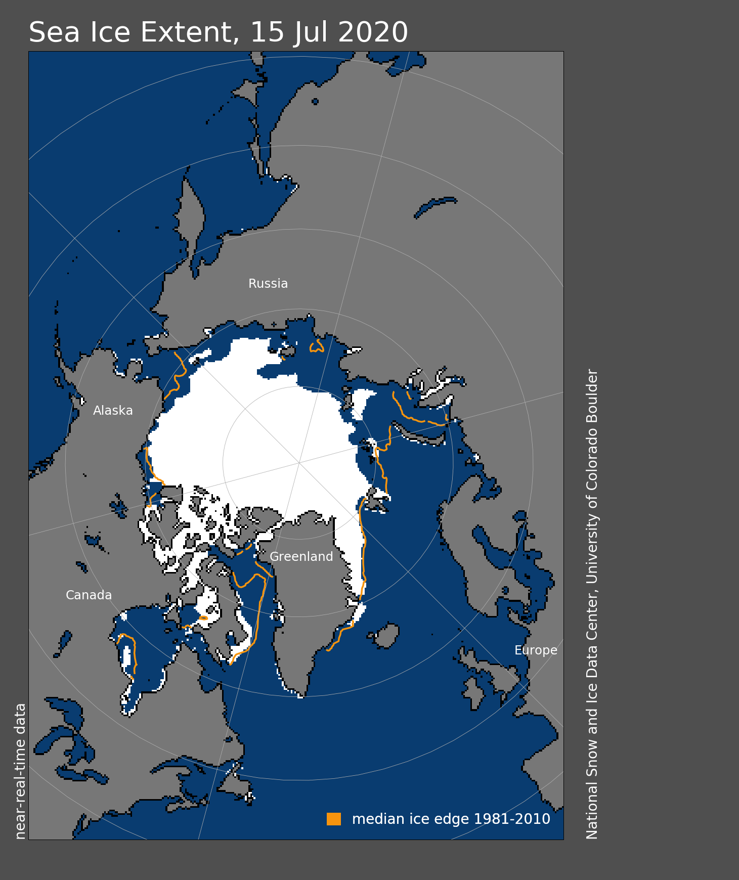
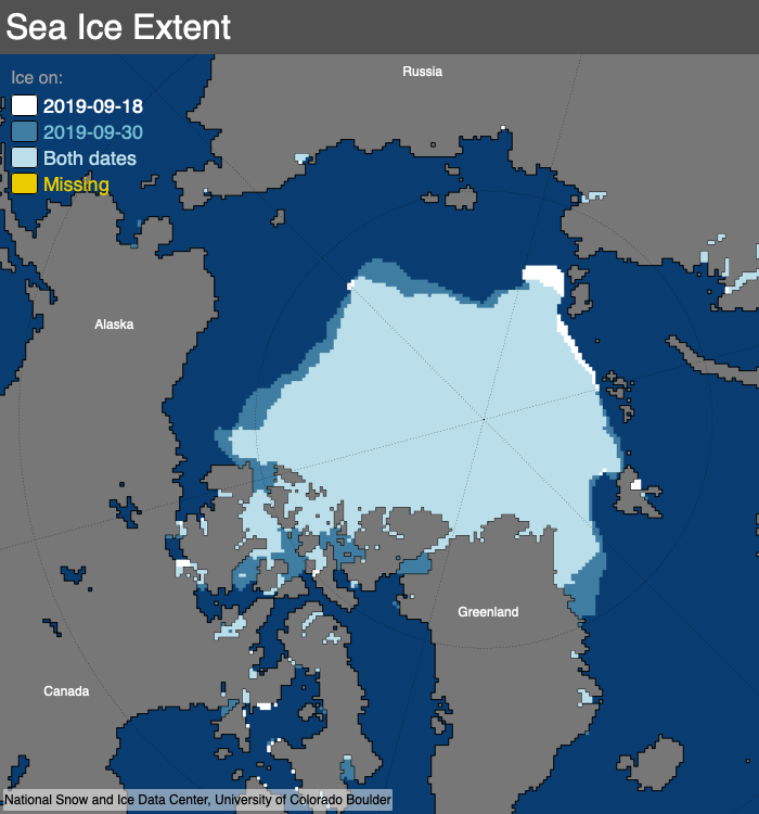
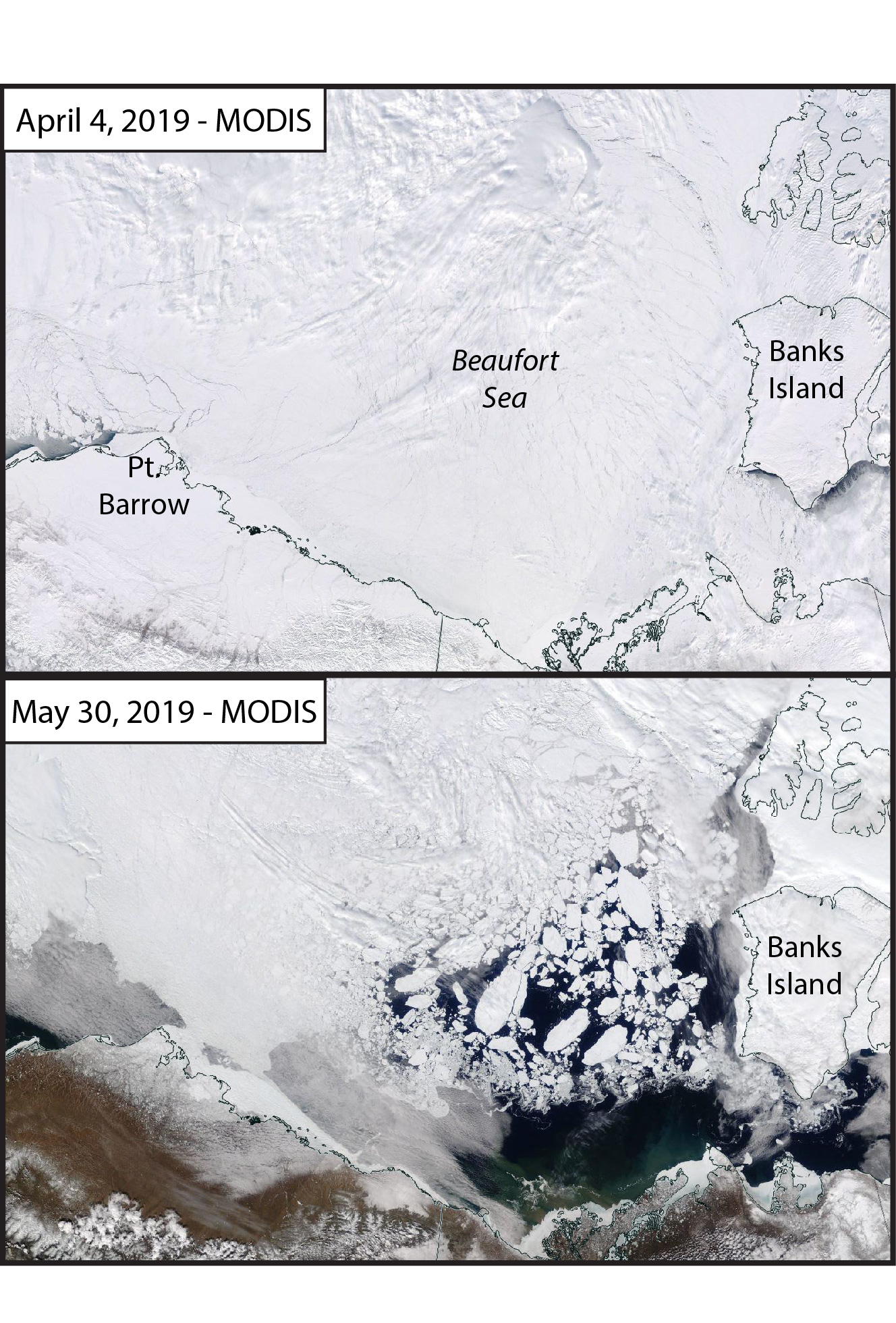
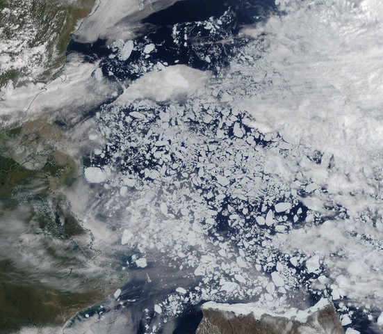
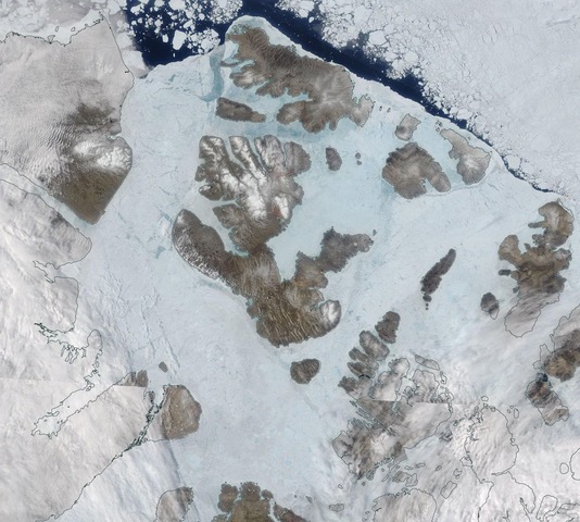
After a period of rapid sea ice loss extending into the last week of August, the rate has slowed with the onset of autumn in the Arctic. A region of low concentration ice persists in the Beaufort Sea. How much of this ice melts over in the next two weeks will strongly determine where the September sea ice minimum will stand in the record books. The Northwest Passage (Amundsen’s route) is largely open but some ice remains. The Northern Sea Route, along the Siberian coast, remains open.

Overview of conditions

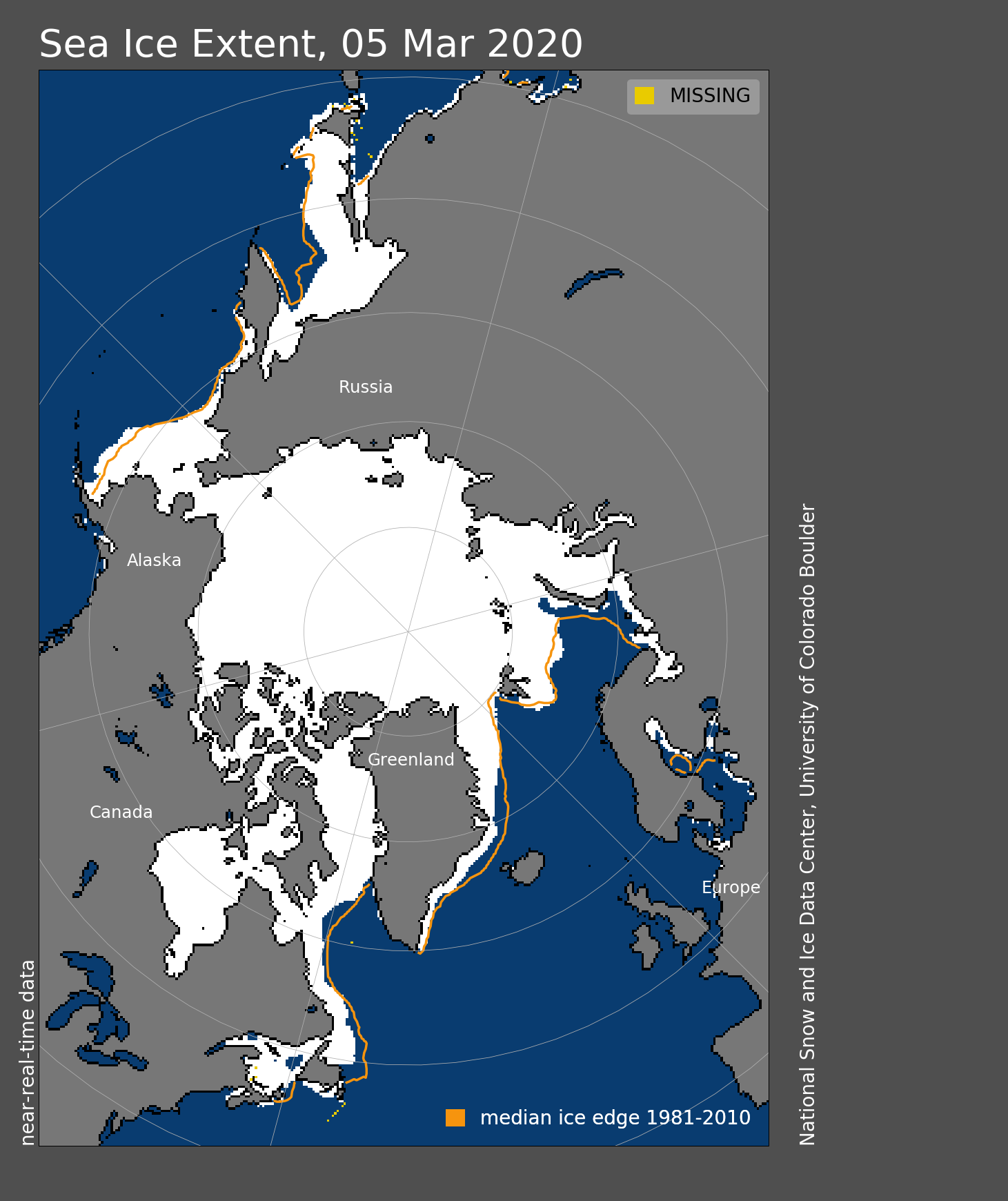
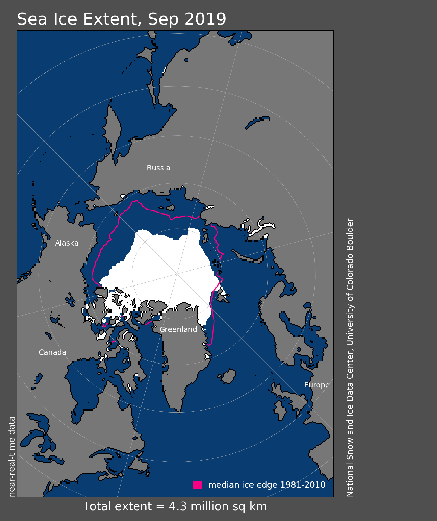
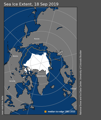
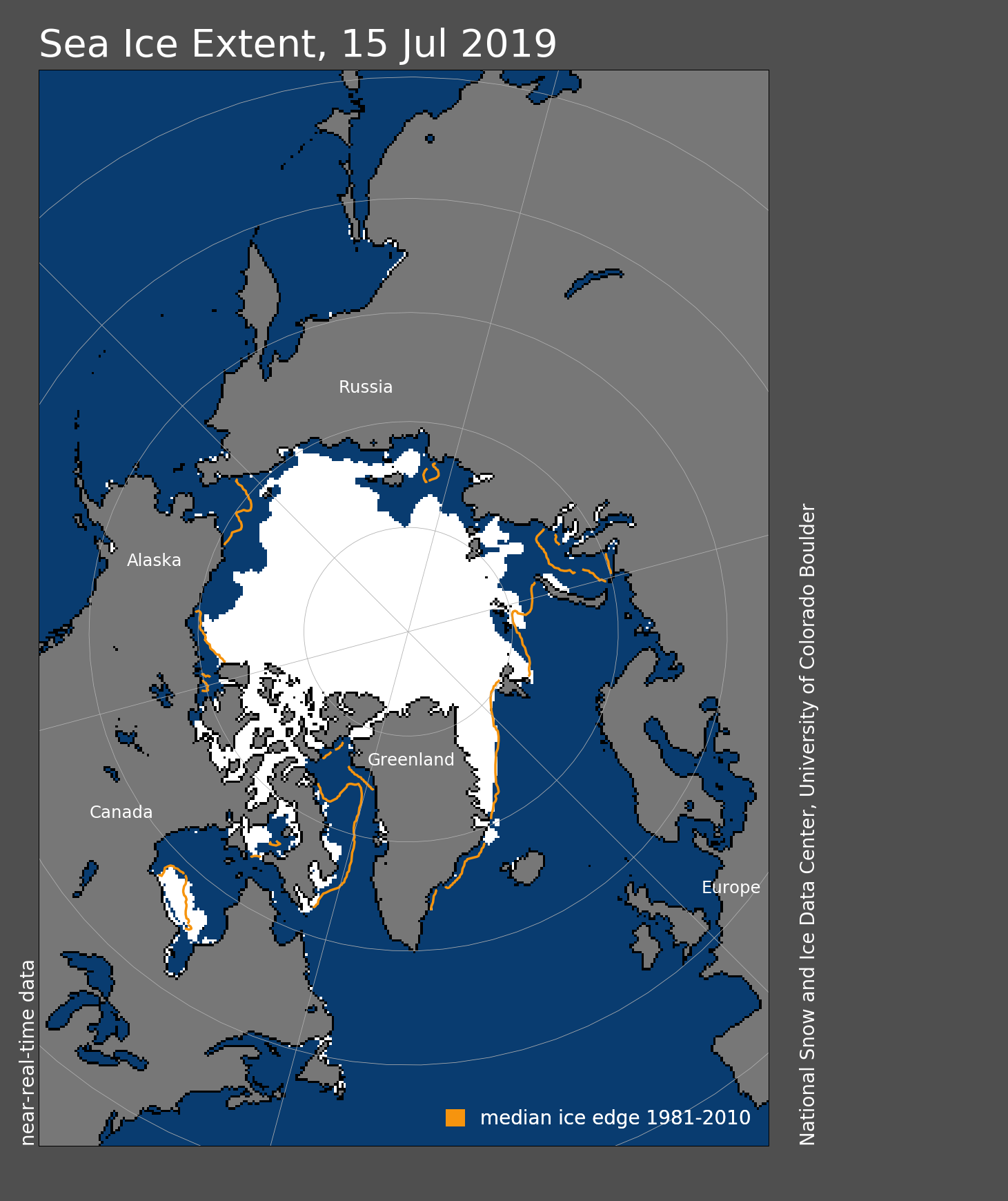
Figure 1. Arctic sea ice extent for August 2020 was 5.08 million square kilometers (1.96 million square miles). The magenta line shows the 1981 to 2010 average extent for that month. Sea Ice Index data. About the data

Credit: National Snow and Ice Data Center
High-resolution image

August 2020 sea ice extent averaged 5.08 million square kilometers (1.96 million square miles), placing it at third lowest in the satellite record for the month. This was 360,000 square kilometers (139,000 square miles) above the record low set in 2012. As of September 1, Arctic sea ice extent stood at 4.26 million square kilometers (1.64 million square miles), the second lowest extent for that date in the satellite passive microwave record that started in 1979.

In our previous post, we noted the development of substantial openings of the sea ice north of Alaska within the Beaufort and Chukchi Seas, possibly related to the mid-July storm that spread out the ice cover. Since then, further melt has occurred in the area. Some of this ice appears to be multiyear, which tends to be resistant to melting away. Total sea ice extent at the September minimum will depend strongly on how much of the ice in this area melts from the remaining heat in the ocean, and on wind compaction or expansion of the overall ice edge (the line of 15 percent concentration). The Northwest Passage is largely open, but some ice remains. The Northern Sea route remains open.

Conditions in context

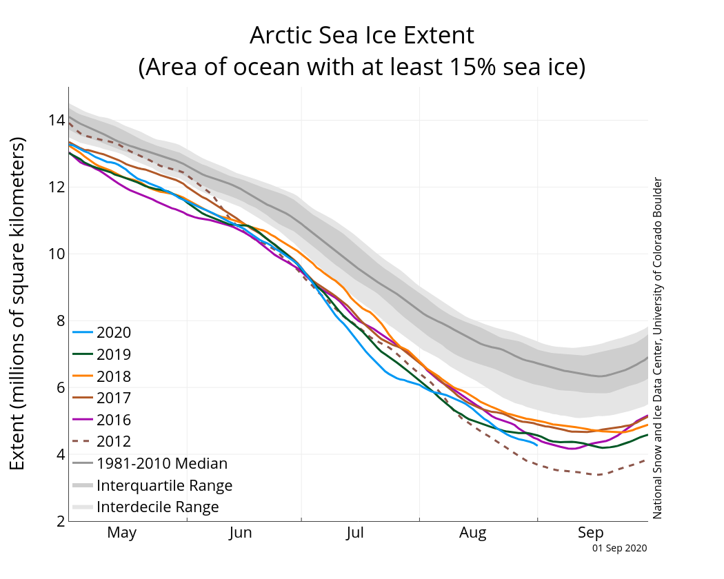
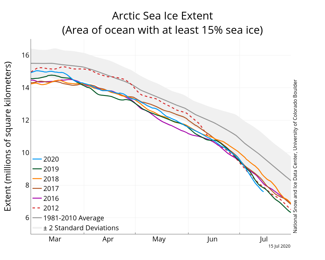
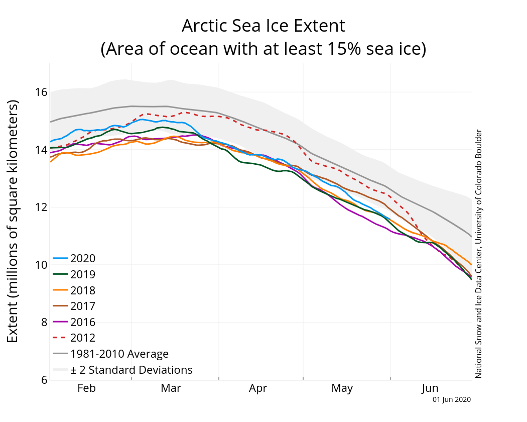
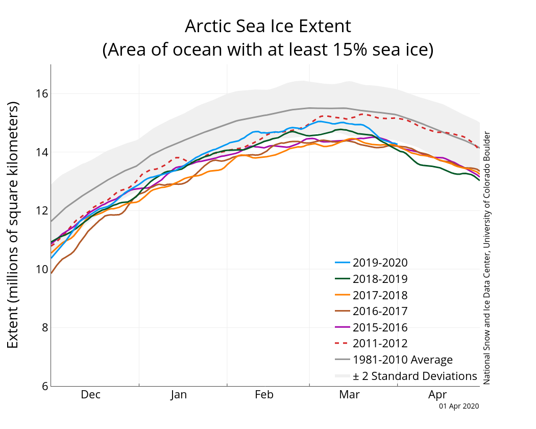
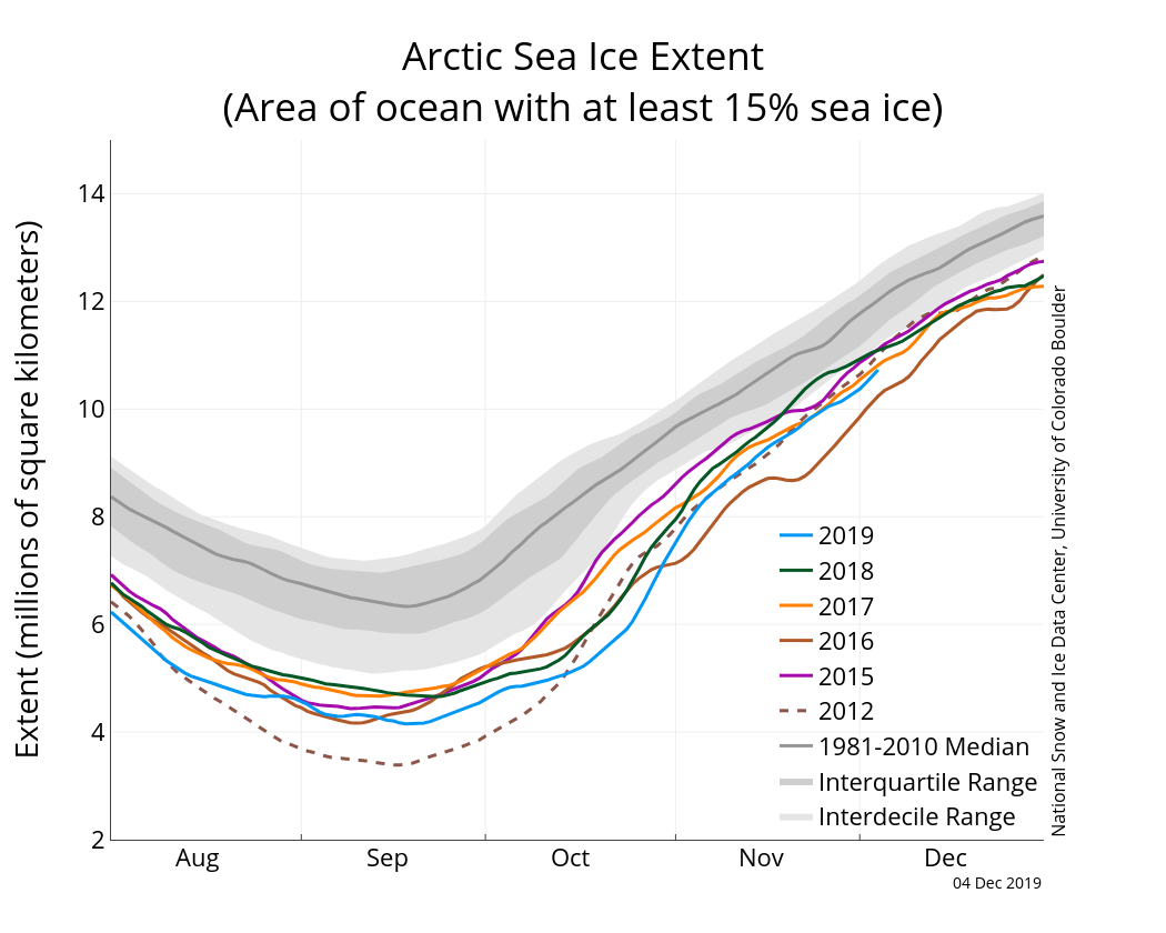
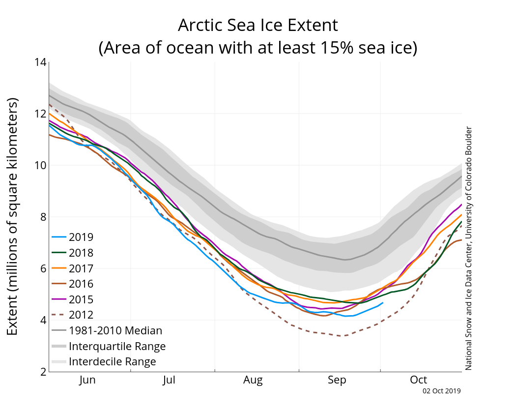
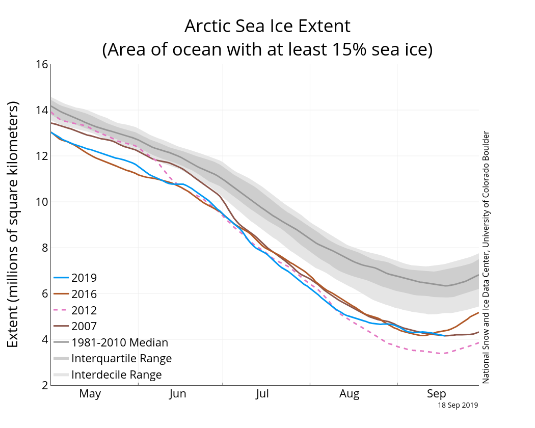
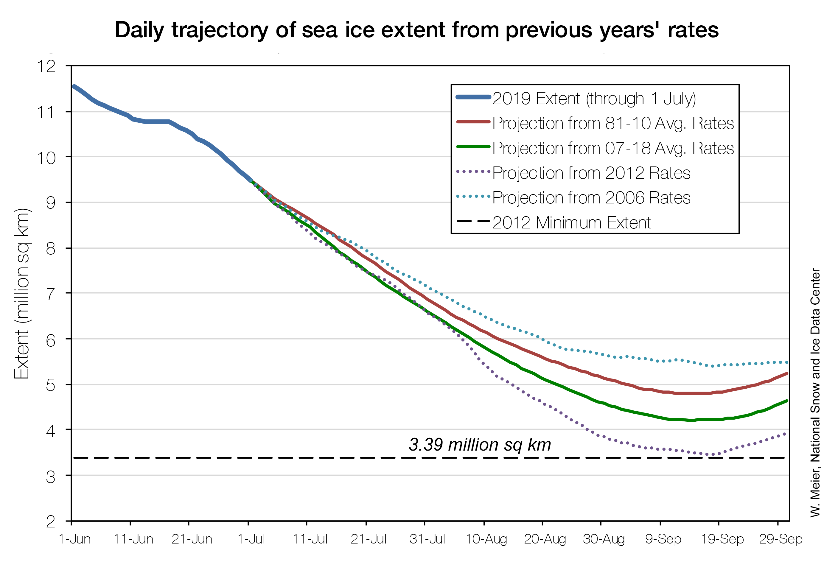
Figure 2a. The graph above shows Arctic sea ice extent as of September 01, 2020, along with daily ice extent data for four previous years and the record low year. 2020 is shown in blue, 2019 in green, 2018 in orange, 2017 in brown, 2016 in purple, and 2012 in dashed brown. The 1981 to 2010 median is in dark gray. The gray areas around the median line show the interquartile and interdecile ranges of the data. Sea Ice Index data.

Credit: National Snow and Ice Data Center
High-resolution image

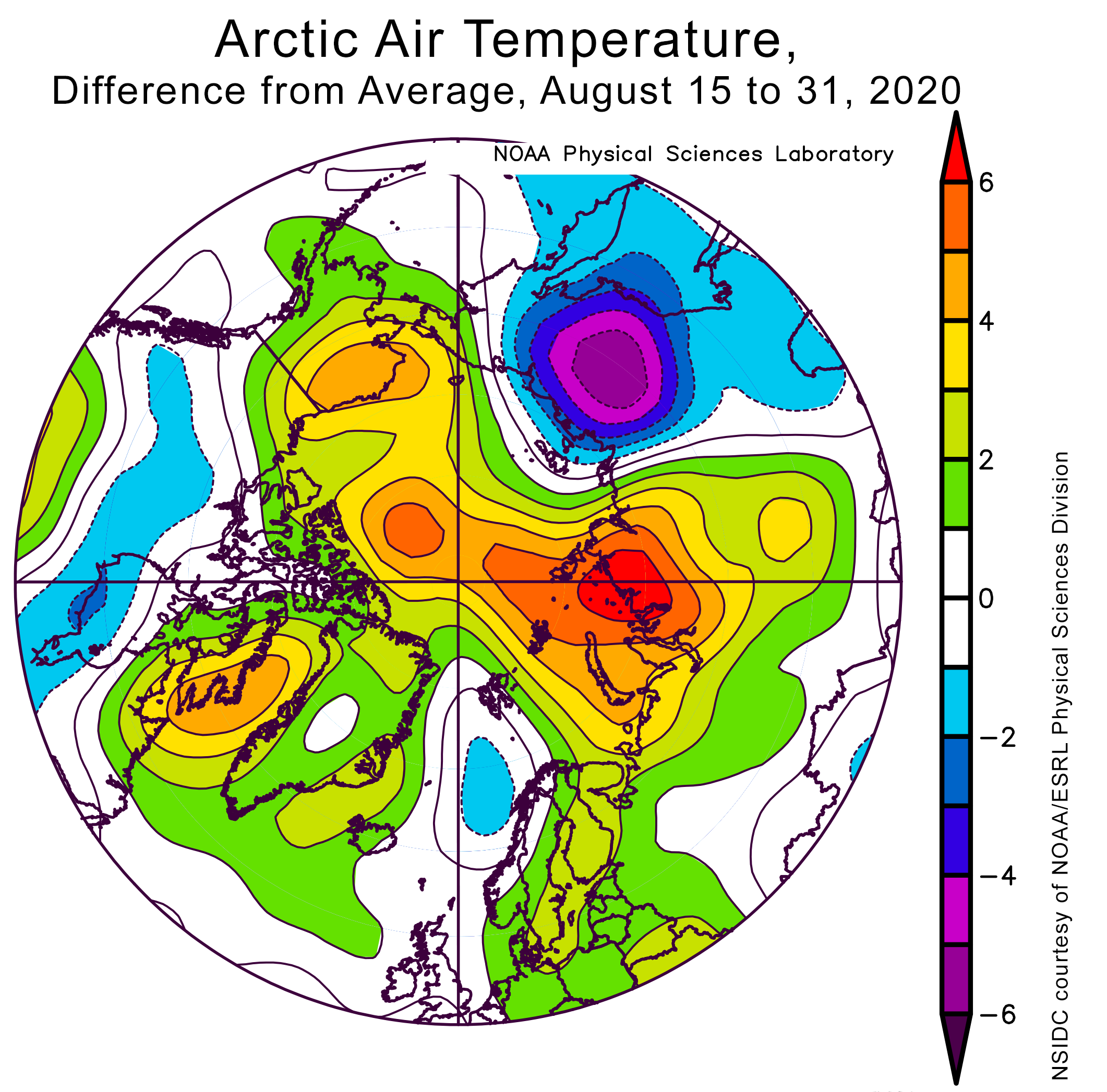
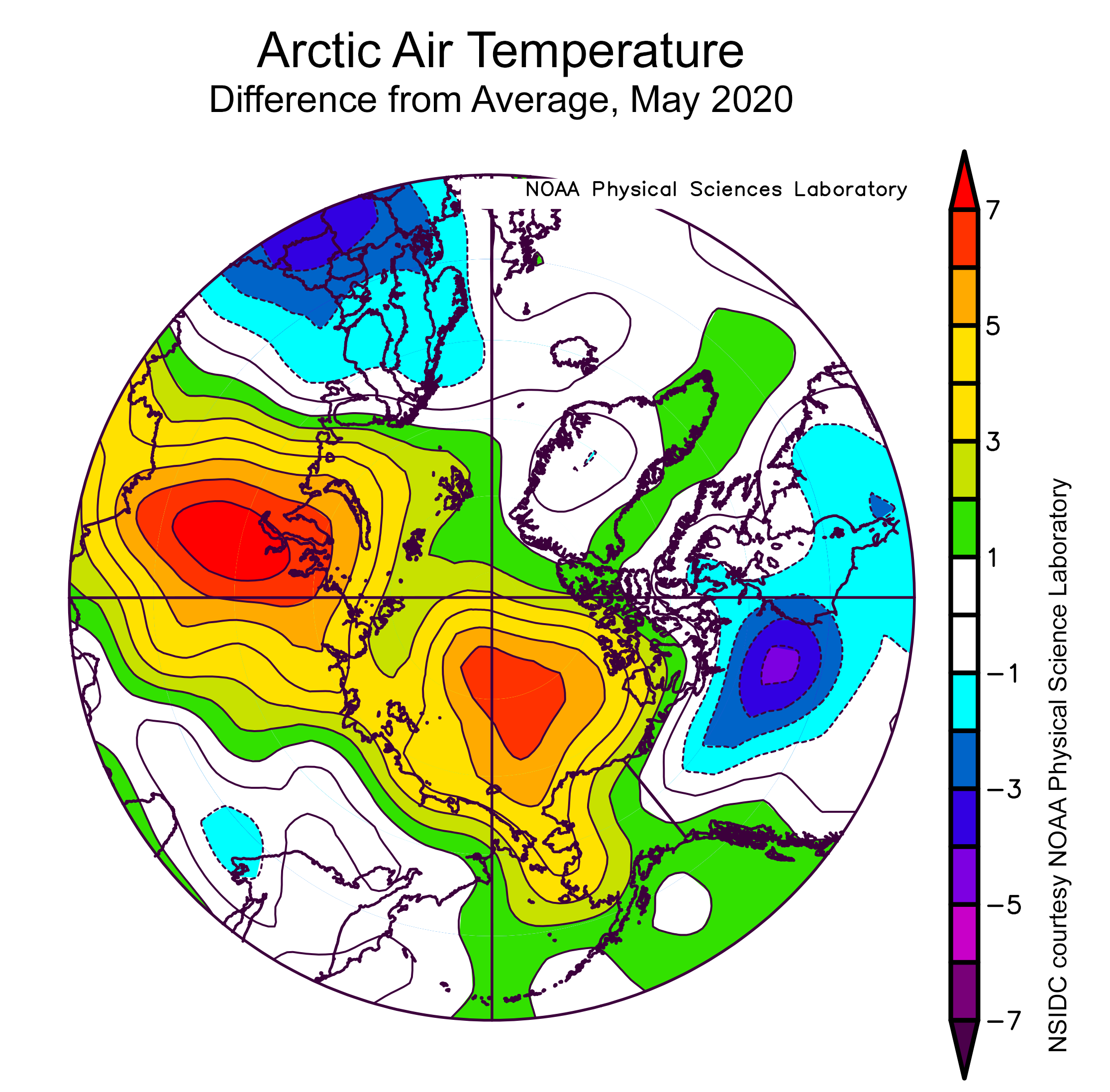
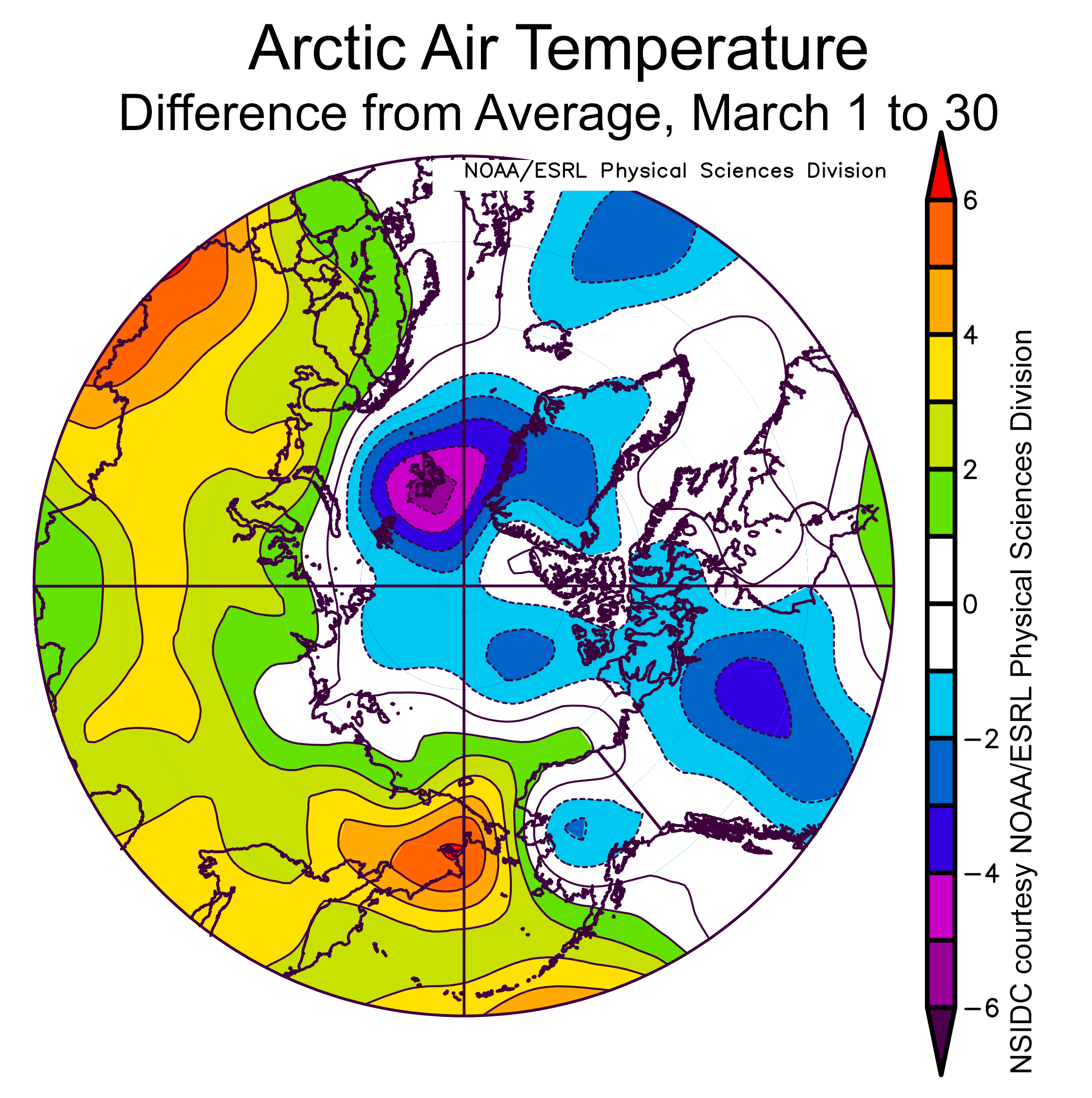
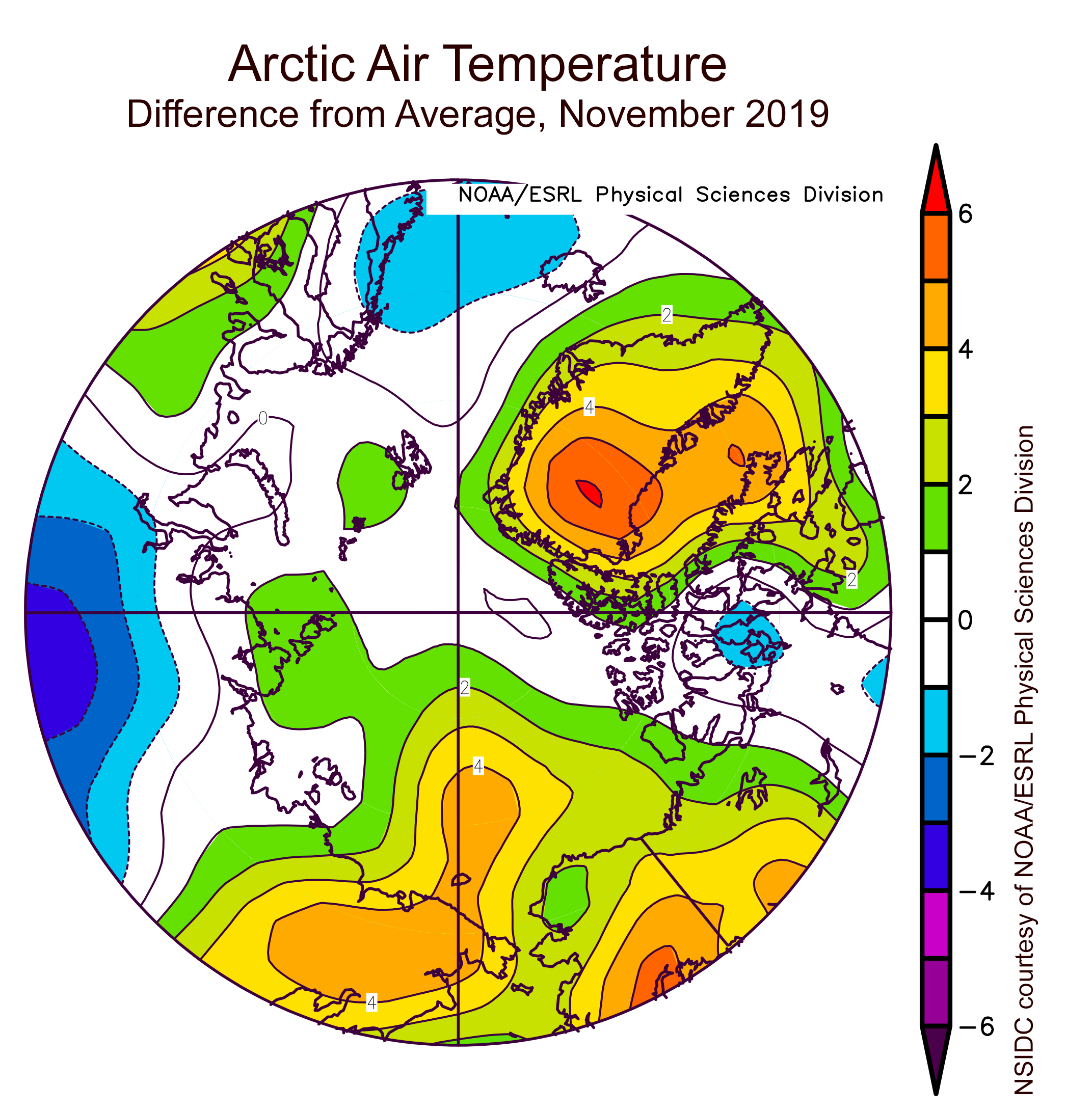
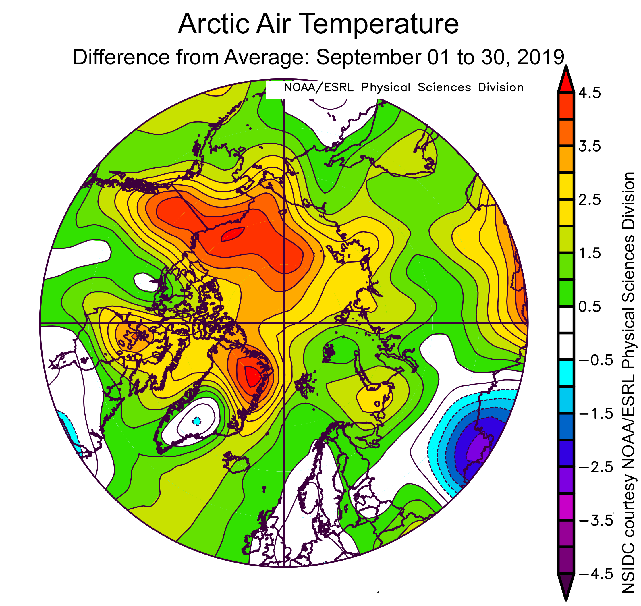
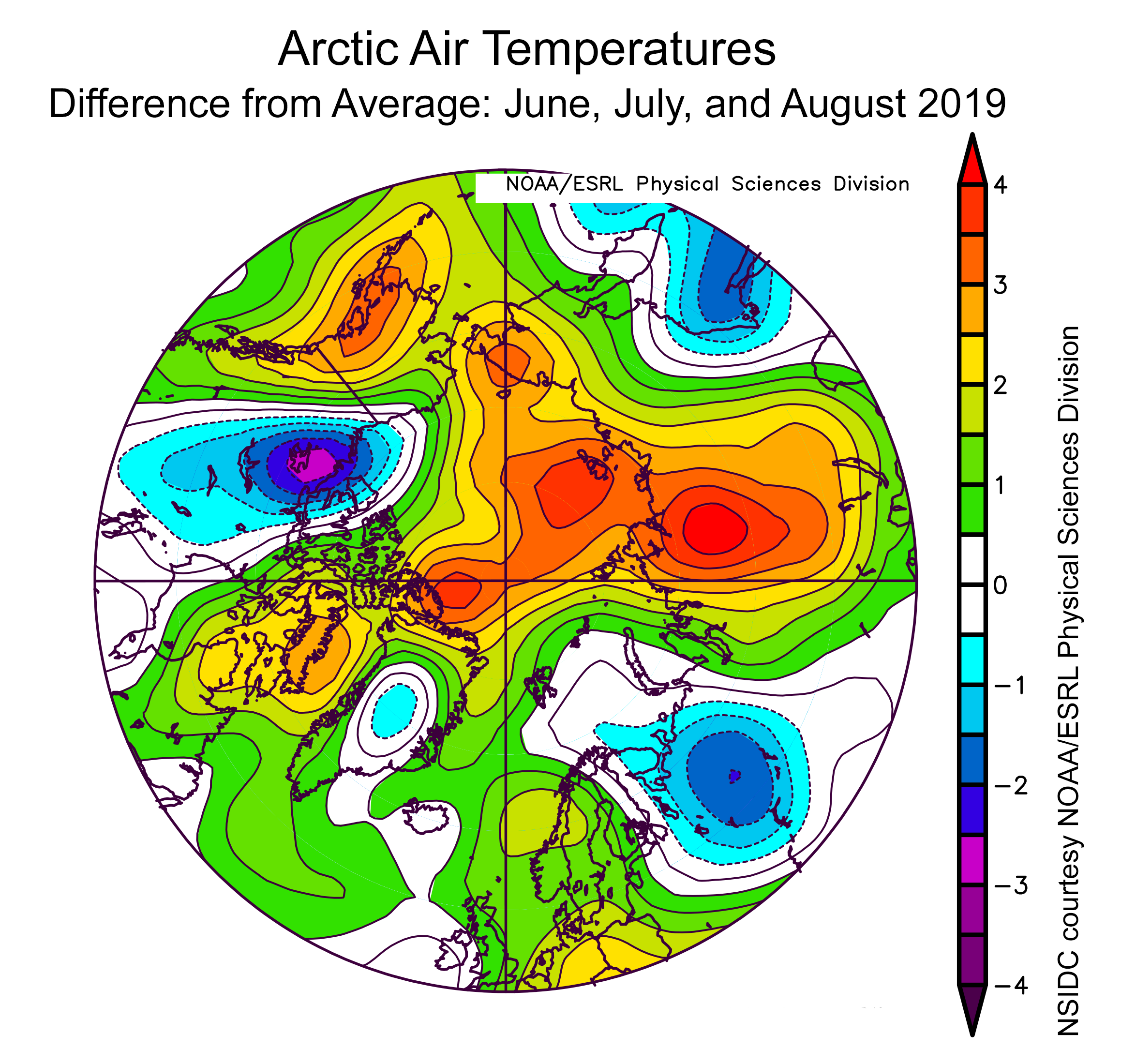
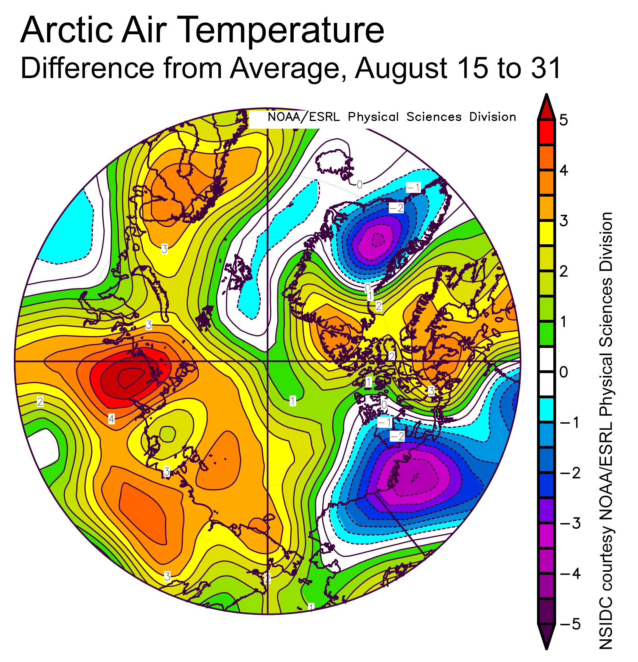
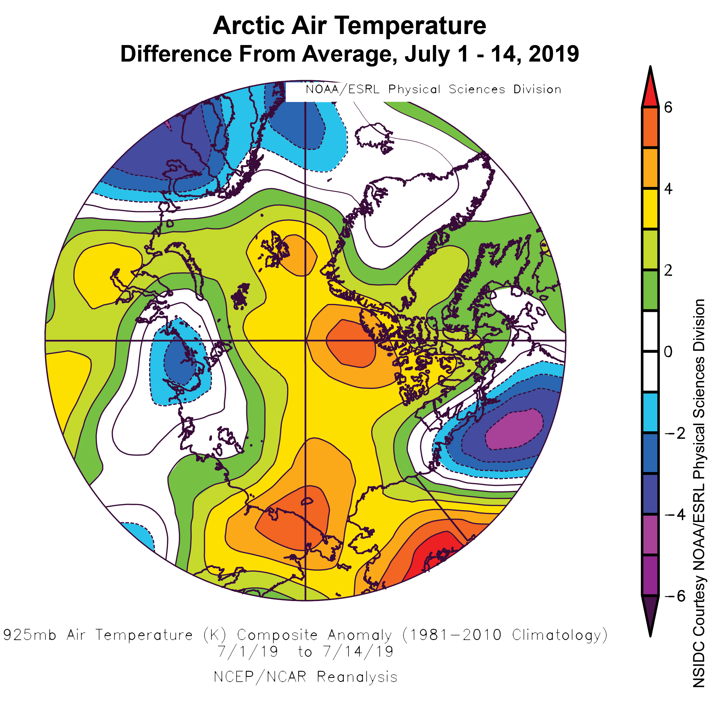
Figure 2b. This plot shows the departure from average air temperature in the Arctic at the 925 hPa level, in degrees Celsius, from August 15 to 31, 2020. Yellows and reds indicate higher than average temperatures; blues and purples indicate lower than average temperatures.

Credit: NSIDC courtesy NOAA Earth System Research Laboratory Physical Sciences Division
High-resolution image

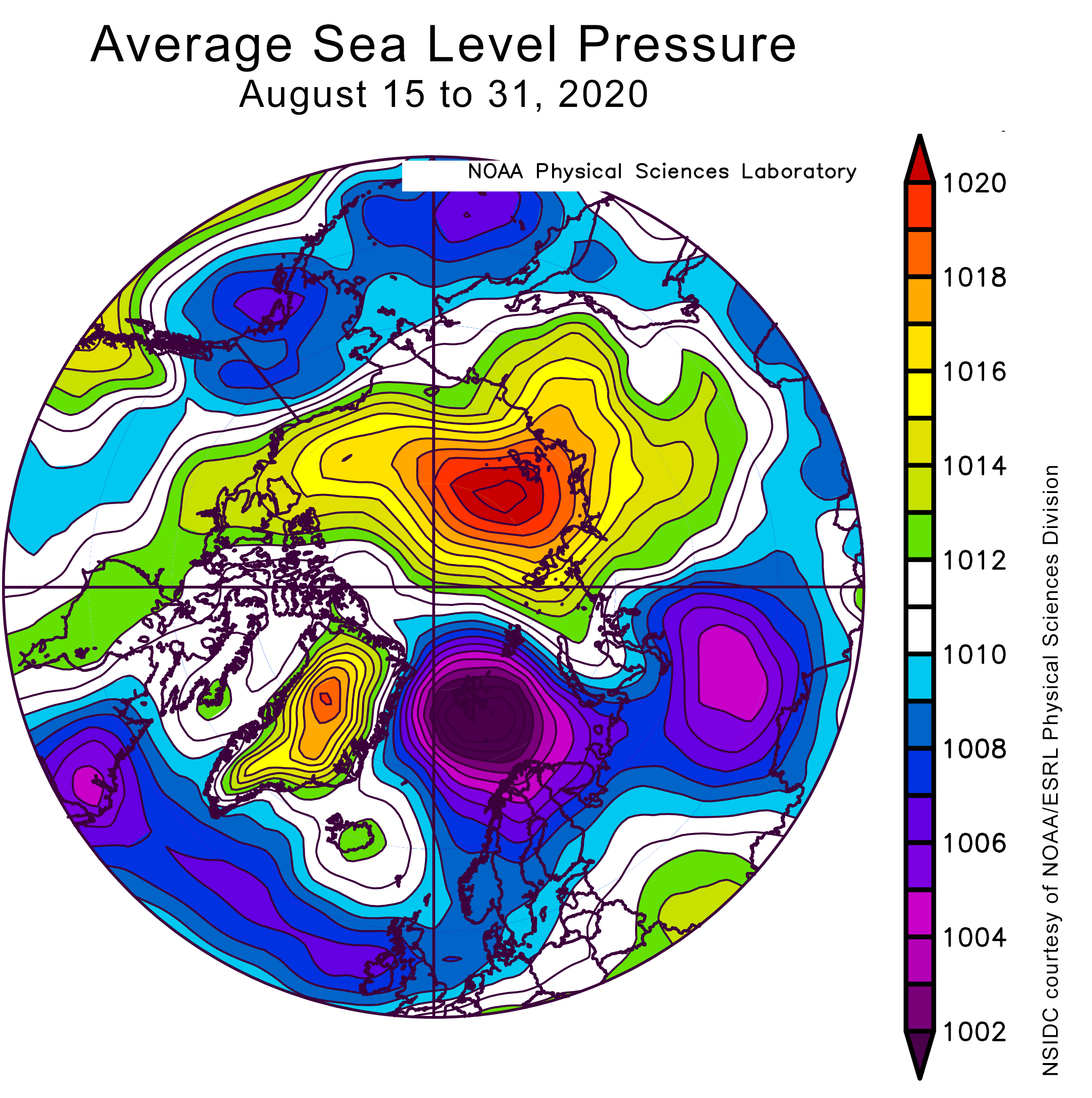
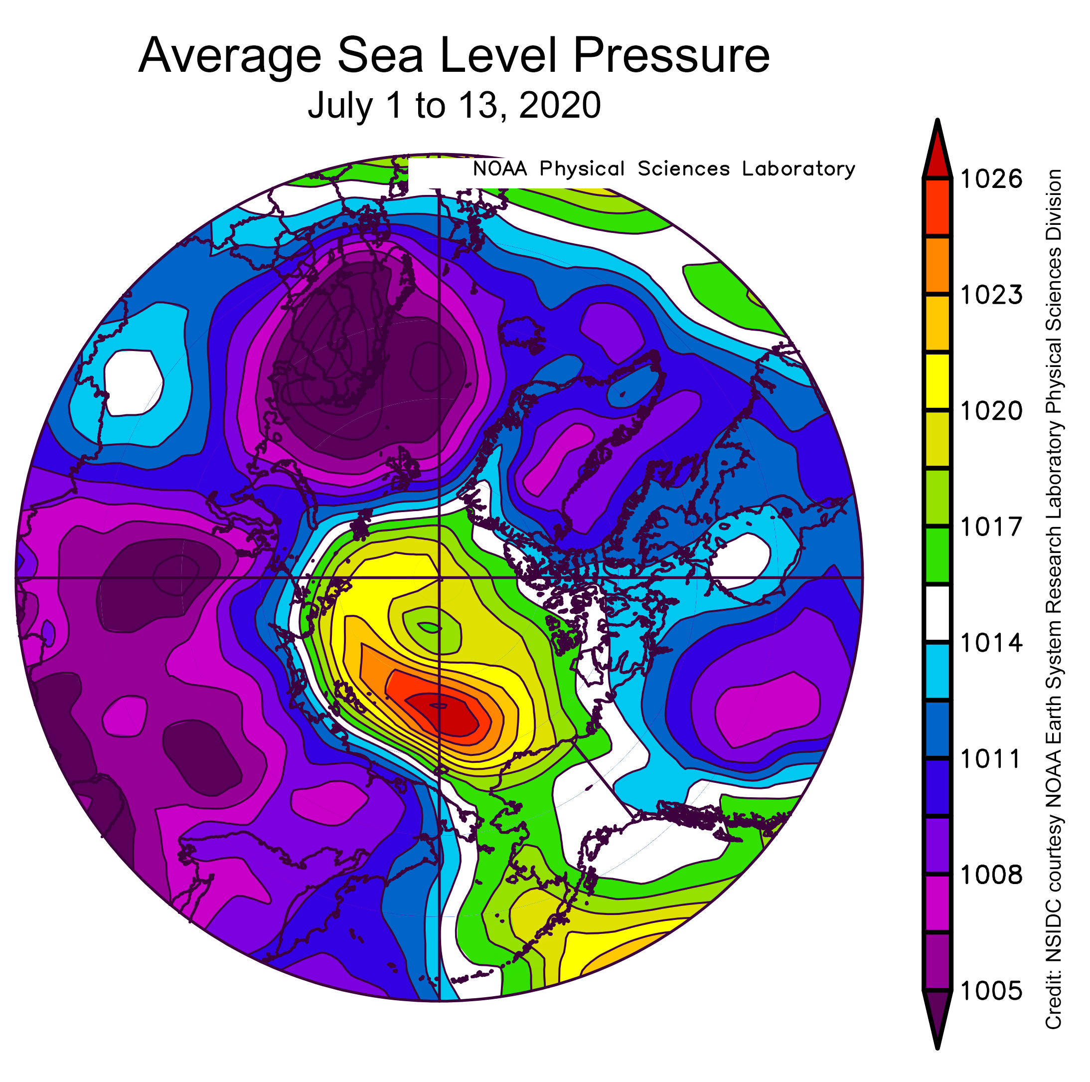
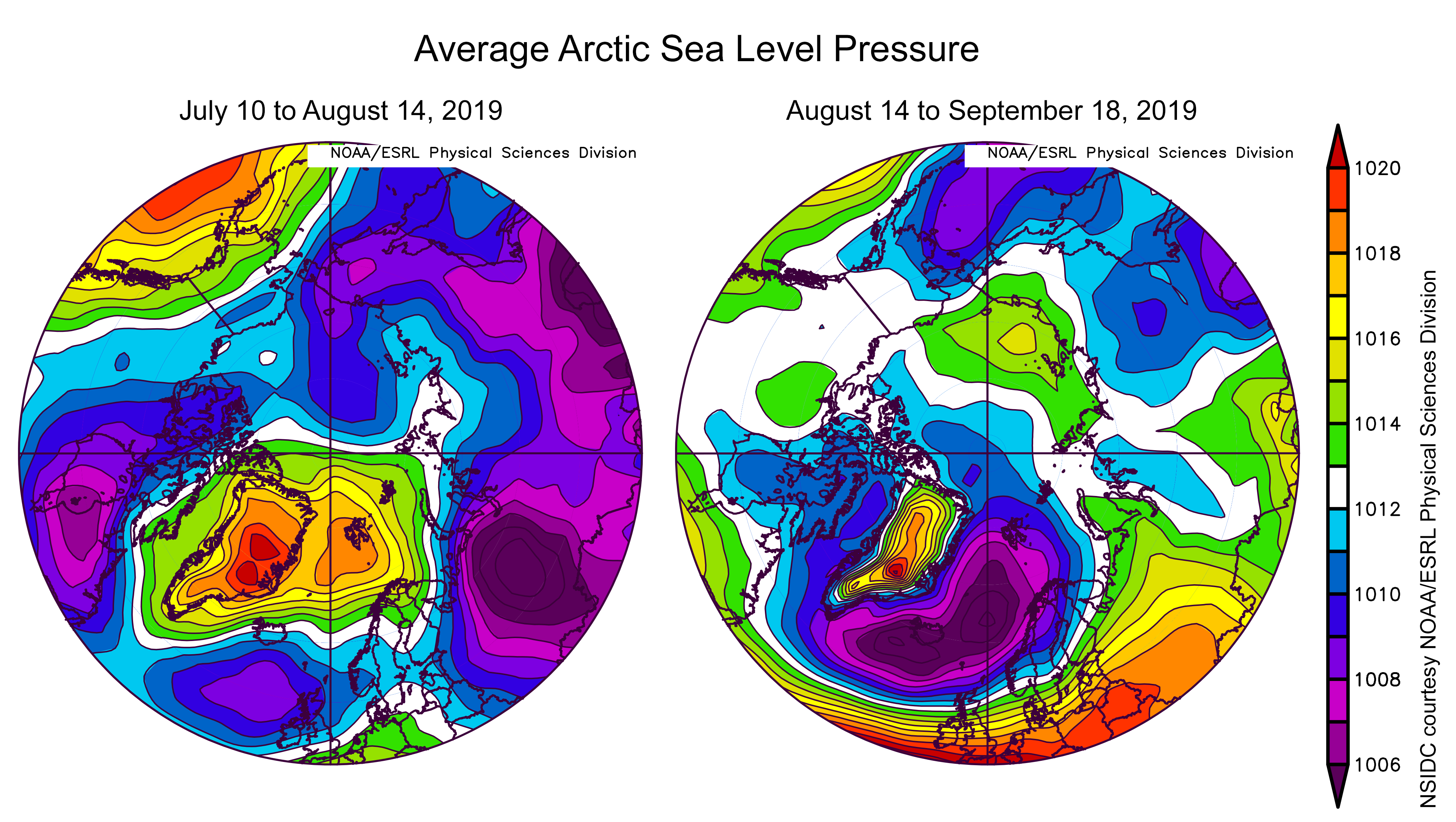
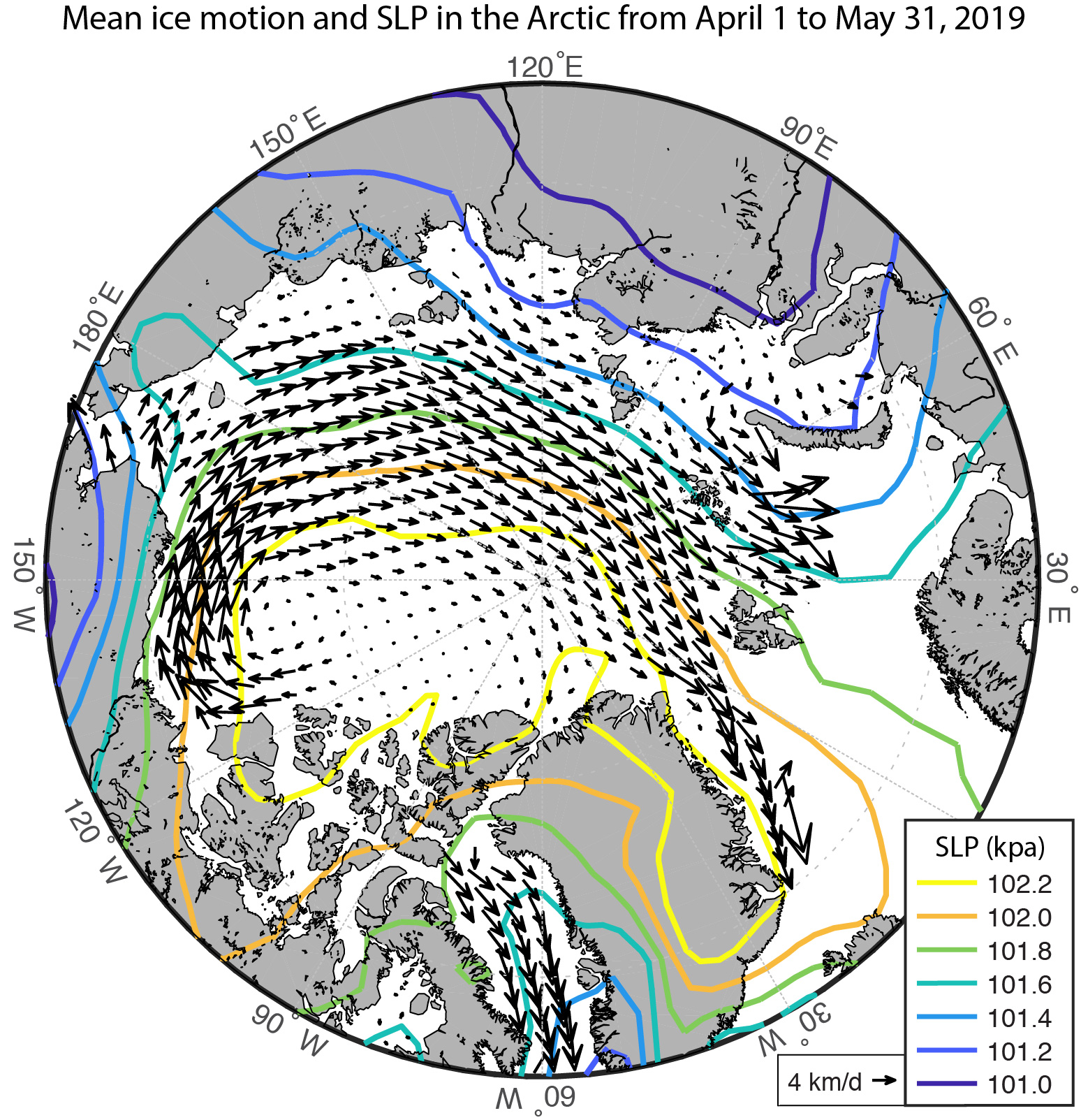
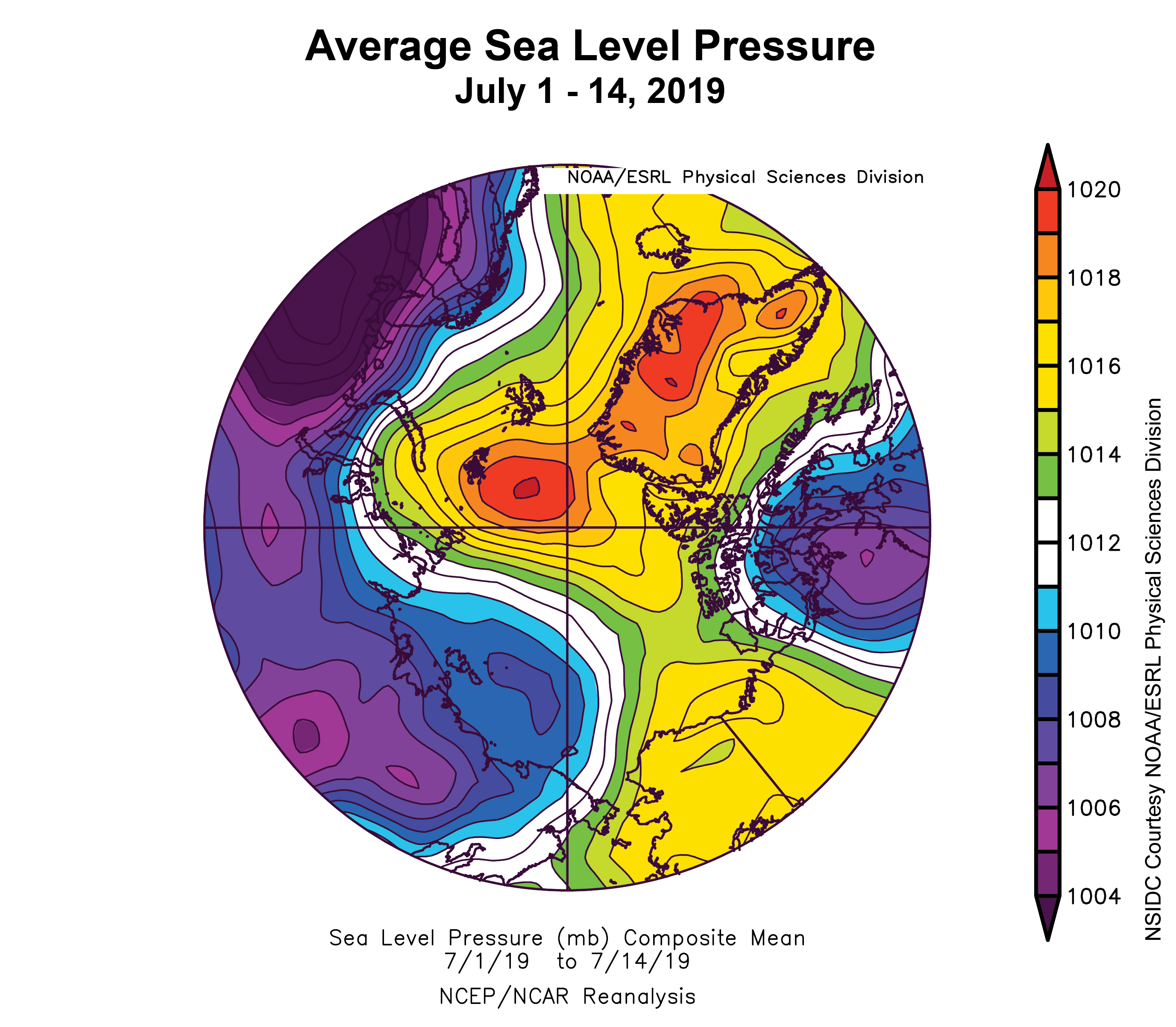
Figure 2c. This plot shows average sea level pressure in the Arctic in millibars (hPa) from August 15 to 31, 2020. Yellows and reds indicate high air pressure; blues and purples indicate low pressure.

Credit: NSIDC courtesy NOAA Earth System Research Laboratory Physical Sciences Division
High-resolution image

Following a period of slow August ice loss, the pace quickened during the middle of the month as areas of low ice concentration melted away, only to slow again towards the end of the month with the onset of autumn in the Arctic. Overall, from August 15 through September 1, 2020, extent declined by 1.1 million square kilometers (425,000 square miles), more than the average 1981 to 2020 extent loss of 800,000 square kilometers (309,000 square miles) during the same period (Figure 2a).

As assessed from August 15 to August 31, air temperatures at the 925 mb level (about 2,500 feet above sea level) were above average over much of the Arctic Ocean, continuing the basic pattern of warmth that prevailed through the first half of the month, most notably in the Kara Sea. Temperatures were below average over central Siberia (Figure 2b). The atmospheric circulation pattern shifted relative to the first half of the month to feature high pressure centered over the Laptev Sea and extending across the Beaufort and Chukchi Seas (Figure 2c). Low pressure has been the dominant feature of the Norwegian Sea region.

August 2020 compared to previous years

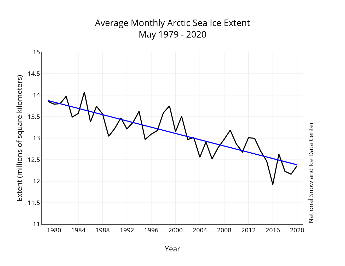
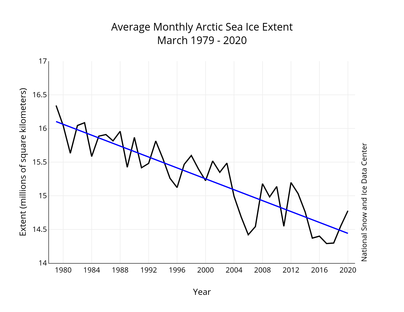
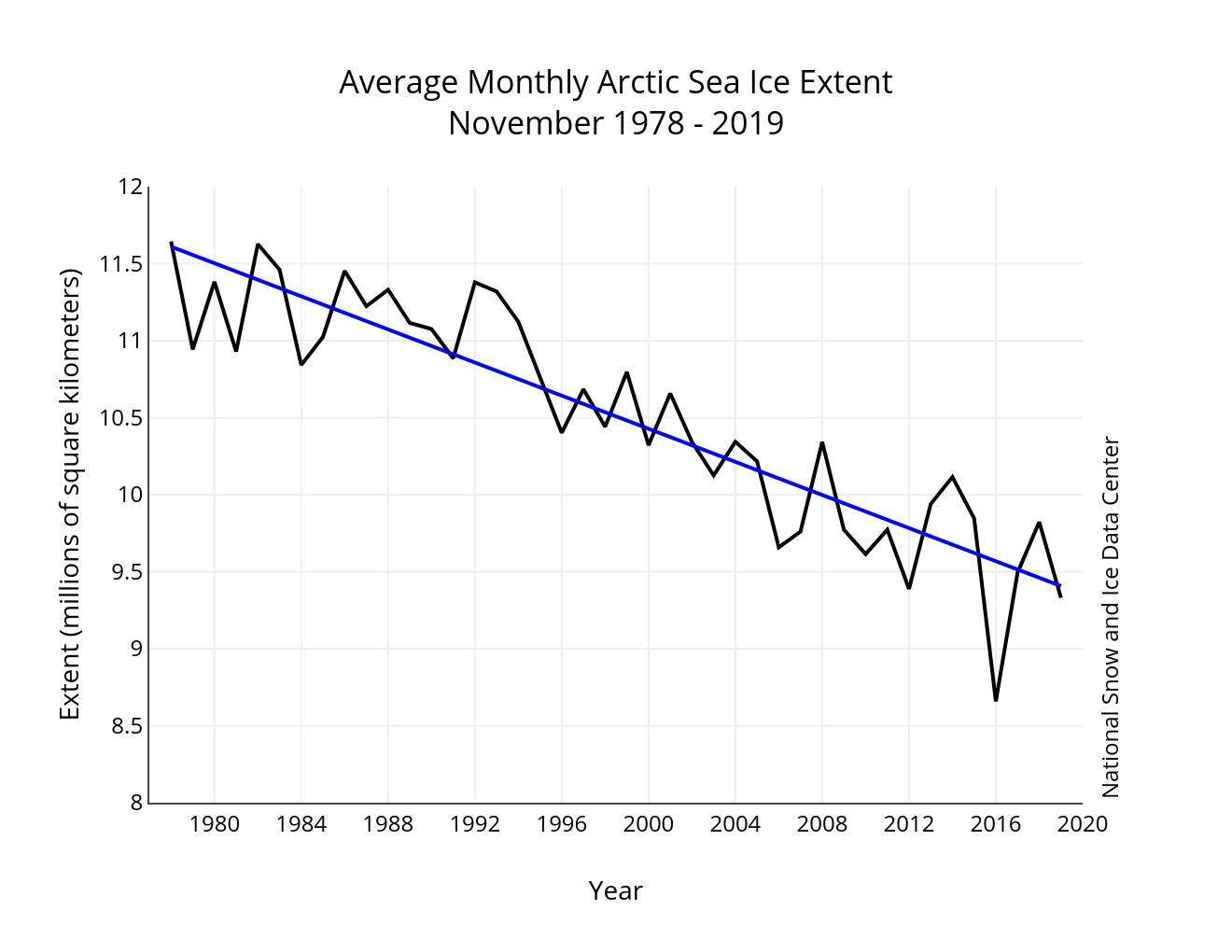
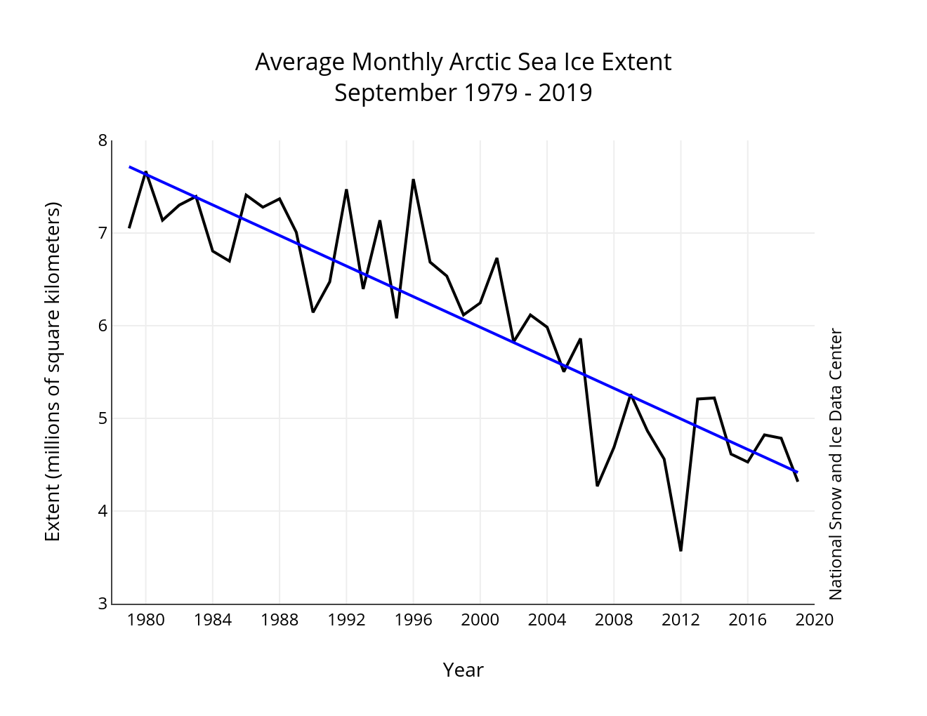
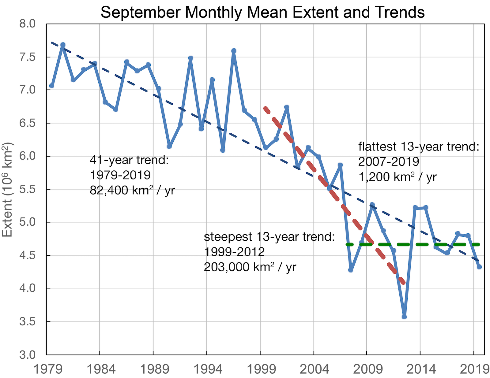
Figure 3. Monthly August ice extent for 1979 to 2020 shows a decline of 10.7 percent per decade.

Credit: National Snow and Ice Data Center
High-resolution image

The average sea ice extent for August 2020 as a whole is 5.08 million square kilometers (1.96 million square miles), placing it third lowest in the 42-year satellite record. Including 2020, the linear rate of decline for August sea ice extent is 10.7 percent per decade. This corresponds to a trend of 76,800 square kilometers (29,700 square miles) per year, or about the size of New Hampshire, Vermont, and Massachusetts combined. Over the satellite record, the Arctic Ocean has lost about 3.15 million square kilometers (1.22 million square miles) of ice in August, based on the difference in linear trend values in 2020 and 1979. This is comparable in size to about twice the size of the state of Alaska.

Atlantification continues

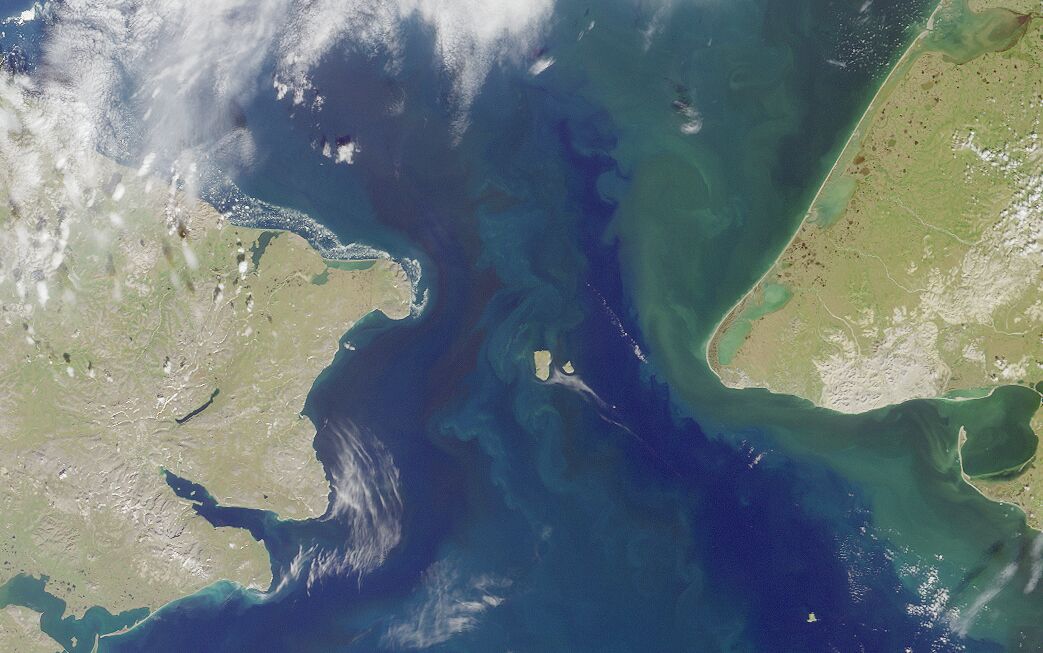
As discussed in a recent paper in the Journal of Climate led by colleague Igor Polyakov of the University of Alaska, the process of “Atlantification” of the Arctic Ocean, first noted in the Barents Sea, is continuing, with significant effects on the sea ice cover during the winter season in the Eastern Eurasian Basin. The relatively fresh surface layer of the Arctic Ocean is underlain by warm, salty water that is imported from the northern Atlantic Ocean. The cold fresh surface layer, because of its lower density, largely prevents the warm, salty Atlantic waters from mixing upwards. However, the underlying Atlantic water appears to have moved closer to the surface in recent years, reducing the density contrast with the water above it. Recent observations show this warm water “blob,” usually found at about 150 meters (492 feet) below the surface, has shifted within 80 meters (263 feet) of the surface. This has resulted in an increase in the upward winter ocean heat flow to the underside of the ice from typical values of 3 to 4 watts per square meter in 2007 to 2008 to greater than 10 watts per square meter from 2016 to 2018. Polyakov estimates that this is equivalent to a two-fold reduction in winter ice growth.

Other recent news

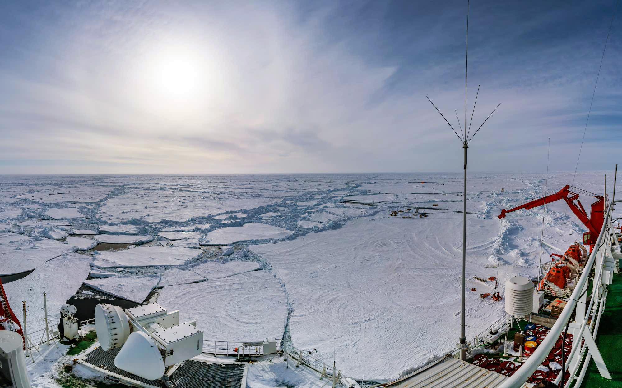
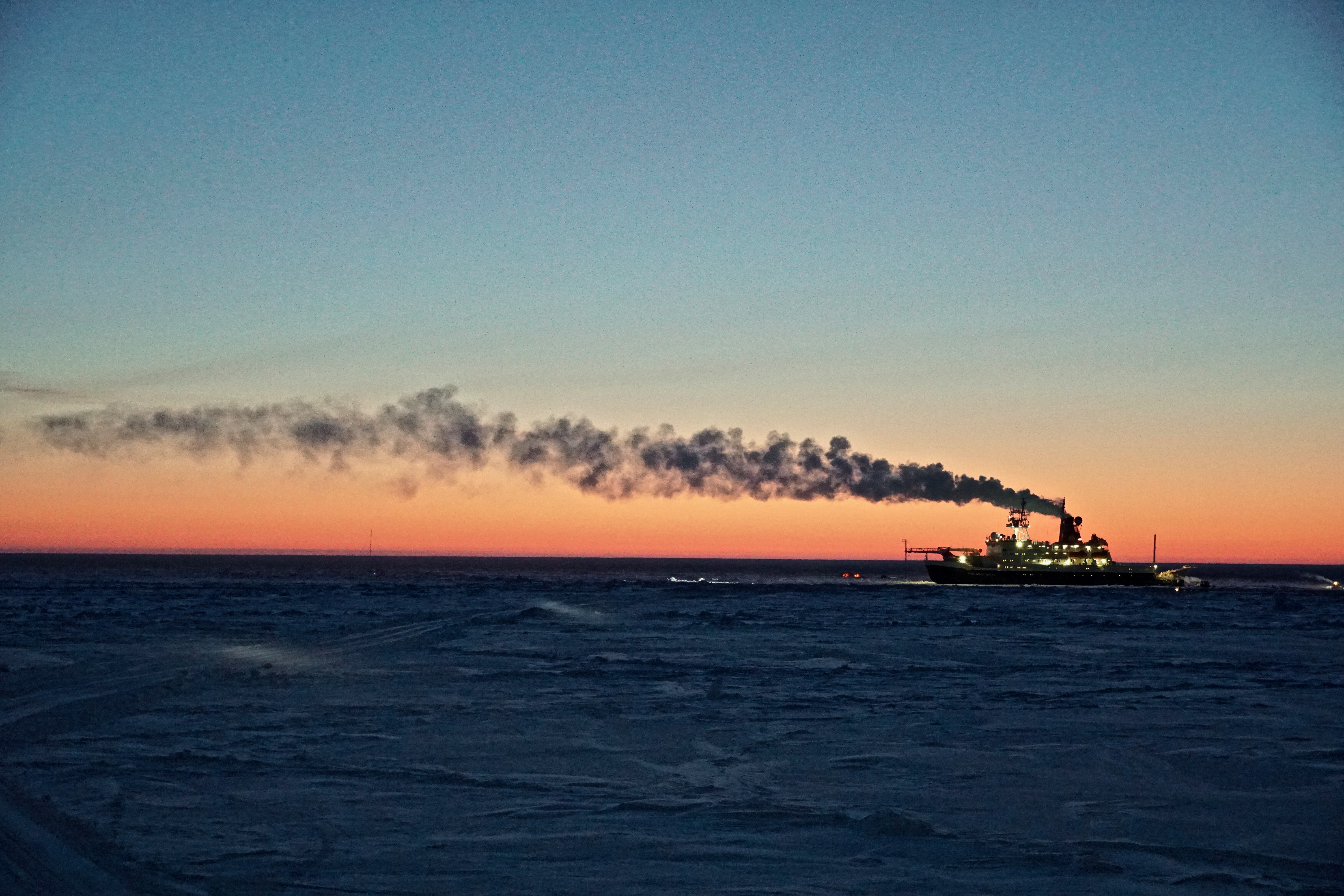
The RV Polarstern, which has been supporting the Multidisciplinary drifting Observatory for the Study of Arctic Climate (MOSAiC) expedition, conducted an impromptu detour to the North Pole, taking advantage of fairly light ice conditions. Large openings in the sea ice were present north of Greenland, an area that would normally be very difficult to traverse. The United States’ medium-duty icebreaker Healy did not fare as well—a fire broke out in the engine compartment, and although it was quickly extinguished, the damage is extensive, and with the ship temporarily out of commission, a planned expedition to the Chukchi and Beaufort Seas has been cancelled.

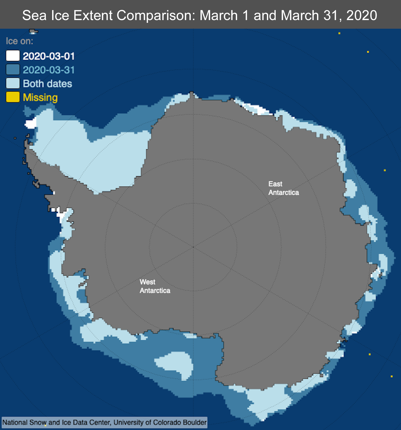
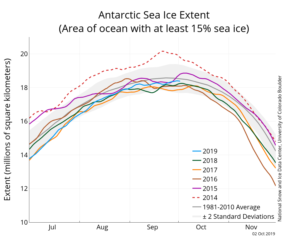
Antarctic sea ice: looking up down below

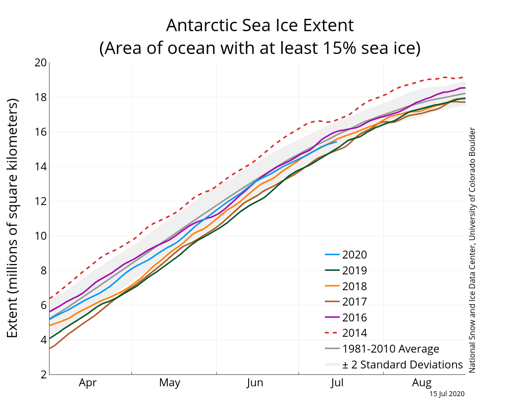
Figure 4. The graph above shows Antarctic sea ice extent as of September 01, 2020, along with daily ice extent data for four previous years and the record maximum extent year. 2020 is shown in blue, 2019 in green, 2018 in orange, 2017 in brown, 2016 in purple, and 2014 in dashed brown. The 1981 to 2010 median is in dark gray. The gray areas around the median line show the interquartile and interdecile ranges of the data. Sea Ice Index data.

Credit: National Snow and Ice Data Center
High-resolution image

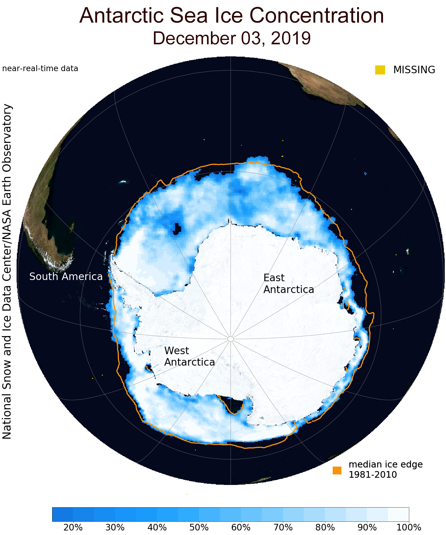
Antarctic sea ice growth in late winter has brought the ice extent substantially above average in late August for the first time in four years. Ice extent exceeded the 1981 to 2010 average over much of the Weddell Sea and off the Wilkes Land coast. A few areas of below-average extent persisted in the Davis Sea (south of Perth, Australia) and the northeastern Ross Sea. The cause appears to be persistent high air pressure in the western Weddell Sea and the Davis Sea that generate offshore cold winds on the eastern sides of the high-pressure areas. While Antarctica often has a trio of high pressure and low pressure areas surrounding it, for the second half of August there were just two such pairs.

Further reading

Polyakov, I. V., et al. 2020. Weakening of Cold Halocline Layer Exposes Sea Ice to Oceanic Heat in the Eastern Arctic Ocean. Journal of Climate, 33, 8107–8123, doi:10.1175/JCLI-D-19-0976.1.

By July 15, 2020, Arctic sea ice extent was at a record low over the period of satellite observations for this time of year. The Siberian heat wave this past spring initiated early ice retreat along the Russian coast, leading to very low sea ice extent in the Laptev and Barents Seas. The Northern Sea route appears to be nearly open.

Overview of conditions

Figure 1. Arctic sea ice extent for July 15, 2020 was 7.51 million square kilometers (2.90 million square miles). The orange line shows the 1981 to 2010 average extent for that day. Sea Ice Index data. About the data

Credit: National Snow and Ice Data Center
High-resolution image

On July 15, Arctic sea ice extent stood at 7.51 million square kilometers (2.90 million square miles), 330,000 square kilometers (127,000 square miles) below the record for July 15, set in 2011. This places extent at the lowest level for this time of year on the satellite record. Low extent for the Arctic as a whole is largely driven by extensive open water in the Laptev and Barents Seas, continuing the pattern that began this spring and was discussed in the previous post. Ice concentrations are low in the East Siberian Sea; remaining ice in this area is likely to melt out soon. By contrast, extent north of Alaska is near the 1981 to 2010 average for this time of year. Such contrasts serve as prominent examples of the larger variations that occur for sea ice extent on the regional scale in comparison to the Arctic Ocean as a whole.

Conditions in context

Figure 2a. The graph above shows Arctic sea ice extent as of July 15, 2020, along with daily ice extent data for four previous years and the record low year. 2020 is shown in blue, 2019 in green, 2018 in orange, 2017 in brown, 2016 in purple, and 2012 in dashed red. The 1981 to 2010 median is in dark gray. The gray areas around the median line show the interquartile and interdecile ranges of the data. Sea Ice Index data.

Credit: National Snow and Ice Data Center
High-resolution image

Figure 2b. This plot shows the departure from average air temperature in the Arctic at the 925 hPa level, in degrees Celsius, from July 1 to 13, 2020. Yellows and reds indicate higher than average temperatures; blues and purples indicate lower than average temperatures.

Credit: NSIDC courtesy NOAA Earth System Research Laboratory Physical Sciences Division
High-resolution image

Figure 2c. This plot shows average sea level pressure in the Arctic in millibars (hPa) from July 1 to 13, 2020. Yellows and reds indicate high air pressure; blues and purples indicate low pressure.

Credit: NSIDC courtesy NOAA Earth System Research Laboratory Physical Sciences Division
High-resolution image

Figure 2d. This true-color composite image shows broken up sea ice on the Siberian coast, taken by the Moderate Resolution Imaging Spectroradiometer (MODIS) sensor on the NASA Terra satellite on July 12, 2020. Also visible is the smoke from wildfires surging in Siberia.

Credit: NASA Worldview
High-resolution image

Through the first half of July 2020, sea ice extent declined by an average of 146,000 square kilometers (56,400 square miles) per day, considerably faster than the 1981 to 2010 average rate of 85,900 square kilometers (33,200 square miles) per day  (Figure 2a).

Air temperatures at the 925 mb level (about 2,500 feet above sea level), as averaged over the first half of July, were unusually high over the central Arctic Ocean—up to 10 degrees Celsius (18 degrees Fahrenheit) (Figure 2b). These above average temperatures were associated with high sea level pressure, centered over the East Siberian and Chukchi Seas (Figure 2c). Arctic temperatures along the Russian coast were near to slightly above average. This is a sharp change from June, when, as part of the Siberian heat wave that has garnered much attention in the media, temperatures along the Siberian coast of the eastern Laptev Sea were 8 degrees Celsius (14 degrees Fahrenheit) above average. It is likely these high temperatures, combined with ice motion away from the coast, initiated early ice retreat along the Russian coast, leading to the present low ice extent (Figure 2d). Based on imagery from AMSR-2 processed by colleagues at the University of Bremen, the Northern Sea Route along the Russian coast appears to be largely open.

Greenland melting

For the first half of July, surface melt over the Greenland Ice Sheet has been above the 1981 to 2010 average, with a spike on July 10 when about 34 percent of the ice sheet experienced some melt. However, this spike pales in comparison to July 11, 2012, when nearly the entire ice sheet experienced some melt. Melt spikes are associated with warm air advection and cloud cover associated with the passage of weather systems. To date, the 2020 season has seen above average surface melt area, relative to 1981 to 2010, but somewhat lower melt extent than several recent years. A further analysis of the ongoing Greenland melt season will be forthcoming in early August in our Greenland Today analysis.

Antarctica freezing

Figure 3. The graph above shows Antarctic sea ice extent as of July 15, 2020, along with daily ice extent data for four previous years and the record high year. 2020 is shown in blue, 2019 in green, 2018 in orange, 2017 in brown, 2016 in purple, and 2014 in dashed red. The 1981 to 2010 median is in dark gray. The gray areas around the median line show the interquartile and interdecile ranges of the data. Sea Ice Index data.

Credit: National Snow and Ice Data Center
High-resolution image

Antarctic sea ice extent as of July 15 was slightly below the 1981 to 2010 average, continuing the trend for nearly every day this year. An effort is underway to use a combination of data from the NASA Ice Cloud and Elevation Satelite-2 (ICESat-2), a laser altimeter, and European Space Agency (ESA) CryoSat-2, a radar altimeter, to provide simultaneous snow surface and underlying sea ice surface heights. Generally, it is assumed that the ICESat-2 laser altimeter estimates the height of the top of the snow, while the radar altimeter on CryoSat-2 penetrates through the snow and obtains a measurement of the top of the ice surface beneath the snow. While there are many uncertainties in these characteristics, subtracting the two values—ICESat-2 height minus CryoSat-2 height—can potentially provide an estimate of snow thickness, a key variable needed to accurately determine sea ice thickness. A study by colleague Ron Kwok demonstrated the efficacy of the approach at cross-over point for the two satellite’s orbit tracks. Plans are now underway to align the satellite orbits such that they fly nearly overlapping profiles over long distances with a very short interval between sensor measurements. This longer comparison area and close time separation will be particularly important for assessing Antarctic sea ice, which has much more variability in ice floe age and origin than Arctic sea ice. It will allow the first careful assessment of Antarctic sea ice mass, and over time, the trend in mass, if any.

Further reading

Kwok, R., Kacimi, S., Webster, M. A., Kurtz, N. T., and A. A. Petty. 2020. Arctic snow depth and sea ice thickness from ICESat‐2 and CryoSat‐2 freeboards: A first examination. Journal of Geophysical Research: Oceans, 125, e2019JC016008. doi:10.1029/2019JC016008.

The seasonal decline of Arctic sea ice extent proceeded at a near-average pace in May. Extent did not approach record lows but remained well below the 1981 to 2010 average. Sea ice extent was notably below average in the Barents and Chukchi Seas, but less so than in recent years. Western Russia and the central Arctic Ocean were unusually warm. Recent research demonstrates a strong link between the persistently positive Arctic Oscillation of last winter and early spring and the record stratospheric Arctic ozone hole. The Multidisciplinary drifting Observatory for the Study of Arctic Climate (MOSAiC) ice floe is breaking up and a new one will most likely have to be found to continue the scientific expedition.

Overview of conditions

Figure 1. Arctic sea ice extent for May 2020 was 12.36 million square kilometers (4.77 million square miles). The magenta line shows the 1981 to 2010 average extent for that month. Sea Ice Index data. About the data

Credit: National Snow and Ice Data Center
High-resolution image

Sea ice extent averaged for May 2020 was 12.36 million square kilometers (4.77 million square miles), placing it in the fourth lowest extent in the satellite record for the month. This was 930,000 square kilometers (359,000 square miles) below the 1981 to 2010 May average and 440,000 square kilometers (170,000 square miles) above the record low mark for May set in 2016. Ice retreat was predominantly in the Bering, Chukchi, Barents and Kara Seas, whereas more modest retreats prevailed in Baffin Bay/Davis Strait, northern Hudson Bay, and the southeastern Greenland Sea. The North Water Polynya also opened up during May. As May came to a close, the ice extent was below average in the Barents and Chukchi Seas, but less so than in recent years. Areas of low extent also included southeastern Greenland, northern Hudson Bay, and northern Baffin Bay. Several coastal polynyas began opening along the Russian coast, a pattern which has been common in recent years. A somewhat larger-than-average opening north of Svalbard appeared in May.

Conditions in context

Figure 2a. The graph above shows Arctic sea ice extent as of June 1, 2020, along with daily ice extent data for four previous years and the record low year. 2020 is shown in blue, 2019 in green, 2018 in orange, 2017 in brown, 2016 in purple, and 2012 in dashed red. The 1981 to 2010 median is in dark gray. The gray areas around the median line show the interquartile and interdecile ranges of the data. Sea Ice Index data.

Credit: National Snow and Ice Data Center
High-resolution image

Figure 2b. This plot shows the departure from average air temperature in the Arctic at the 925 hPa level, in degrees Celsius, for May 2020. Yellows and reds indicate higher than average temperatures; blues and purples indicate lower than average temperatures.

Credit: NSIDC courtesy NOAA Earth System Research Laboratory Physical Sciences Division
High-resolution image

Through the month, sea ice declined by an average of 54,100 square kilometers (20,900 square miles) per day, slightly faster than the 1981 to 2010 average of 47,000 square kilometers (18,000 square miles) per day. The total sea ice loss during May 2020 was 1.68 million square kilometers (649,000 square miles).

Air temperatures at the 925 hPa level (about 2,500 feet above the surface) were above average over almost all of the Arctic Ocean, with departures as much as 7 degrees Celsius (13 degrees Fahrenheit) over the central Arctic Ocean (Figure 2b). Temperatures were also up 7 degrees Celsius (13 degrees Fahrenheit) over the western portion of Russia. Far northern Canada had temperatures on the order of 3 to 5 degrees Celsius (5 to 9 degrees Fahrenheit) below average.

Sea level pressures were especially low over Scandinavia, driving winds from south to north toward the Ob River estuary and Kara Sea region was unusually warm. Pressures were quite high over the Canadian Arctic Archipelago.

May 2020 compared to previous years

Figure 3. Monthly May ice extent for 1979 to 2020 shows a decline of 2.7 percent per decade.

Credit: National Snow and Ice Data Center
High-resolution image

Including 2020, the linear rate of decline for May sea ice extent is 2.7 percent per decade. This corresponds to a trend of 36,400 square kilometers (14,100 square miles) per year, or about the size of the state of Indiana. Over the 42-year satellite record, the Arctic has lost about 1.36 million square kilometers (525,000 square miles) of ice in May, based on the difference in linear trend values in 2019 and 1979. This is comparable to about twice the size of the state of Alaska.

Arctic ozone hole and Arctic Oscillation

Figure 4. Arctic stratospheric ozone reached its record low level of 205 Dobson units, shown in blue and turquoise, on March 12, 2020.

Credit: NASA
High-resolution image

As noted in our previous post, the Arctic Oscillation (AO), a key pattern of atmospheric variability over the Arctic and northern Atlantic, was in a persistently positive (cyclonic) phase from mid-December through early spring. Such persistence, which ended only in early May, is highly unusual, and appears to be linked to a strong, cold stratospheric polar vortex and the largest Arctic stratospheric ozone hole observed to date (Figure 4). Scientists have learned there are two-way relationships—what happens in the stratosphere (high in the atmosphere) influences what happens in the lower atmosphere (the troposphere), and vice versa. A study by University of Colorado researcher Zac Lawrence and National Oceanic and Atmospheric Administration (NOAA) researchers Judith Perlwitz and Amy Butler, submitted recently to the Journal of Geophysical Research, took a close look at these connections. They find that the winter of 2019 to 2020 featured an exceptionally strong and cold stratospheric polar vortex. In general, atmospheric waves generated in the troposphere spread both outward and upward into the stratosphere where they can disturb and weaken the stratospheric polar vortex. But this wave activity was fairly weak this past winter, so the vortex remained largely undisturbed. The vortex was also configured in a way such that upward propagating waves were “reflected” back downwards, which further enabled the vortex to remain strong and cold. The end result is that the cyclonic (counterclockwise) circulation at the surface associated with the positive AO was tied closely to the cyclonic circulation of the strong, cold stratospheric vortex. The cold conditions in the stratosphere and its persistence into spring in turn provided favorable conditions to form polar stratospheric clouds, which foster ozone loss through well-understood chemical processes.

MOSAiC turns into a mosaic

Figure 5a. Before the RV Polarstern left its ice floe location to exchange crew and scientists for the next leg of the MOSAiC (Multidisciplinary drifting Observatory for the Study of Arctic Climate) expedition, ice break ups around the ship intensified.

Credit: C. Rohleder
High-resolution image

Figure 5b. A tent compresses under the pressure of Arctic sea ice ridging, showing increased instability in the region surrounding the RV Polarstern. Surface melt appears at the forefront of the image.

Credit: J. Schaffer
High-resolution image

Scientists on leg three of the Multidisciplinary drifting Observatory for the Study of Arctic Climate (MOSAiC) expedition left their ice floe, which was specifically selected for having survived one summer melt season, on May 16 to exchange crew and scientists and pick up cargo from transport vessels in Svalbard. Before the RV Polarstern ship actually departed, scientists hoped to leave behind several instruments that began monitoring ice, ocean, and atmospheric conditions back in October 2019 when the Central Observatory around the ship was initially established. Some of these instruments included autonomous light stations that measure the amount of light under the ice and changes in water color caused by phytoplankton growth. However, as the scientists were getting ready to leave, the ice floe began to break apart, rendering the MOSAiC floe into a true mosaic of ice blocks (Figure 5a and 5b). With such unstable conditions, all of the instrumentation used to provide calibration and validation data for overflights of satellites and aircraft were removed temporarily. It is not clear how many of the instruments left behind will survive, including the light stations. The warming and power hut from the remote sensing site, for instance, was left on the ice and was in a precarious situation as cracks in the ice opened nearby. In more recent days, images from cameras left behind indicate that the surface is melting which will likely make the floe more unstable. Given these conditions, it remains unclear whether or not the MOSAiC expedition will need to find a new floe to continue the experiment through September 2020.

Effects of cyclones on sea ice

Figure 6. These maps of the Arctic Ocean compare sea ice concentration changes four days after cyclonic storms were present to changes that occur when no storms are present. MAM stands for March-April-May; JJA stands for June-July-August; SON is September-October-November; and DJF is December-January-February. Blue tint indicates greater sea ice concentration after a cyclone; the dots indicate areas where the change is different than random variations in sea ice conditions.

Credit: E. Schreiber, University of Colorado Boulder
High-resolution image

A recently-published study by University of Colorado Boulder doctoral candidate Erika Schreiber considered the effects of the passage of Arctic low pressure systems (extratropical cyclones) on sea ice concentration. In earlier studies, a range of effects has been attributed to storms. Some point to increasing sea ice concentration locally, while others argue that winds associated with cyclones disperse the ice. Schreiber’s research shows that, overall, the thermodynamic effects (cold air, snow, and cloudiness) associated with storms increase sea ice concentration in impacted areas days after the storm hit (Figure 6). In warm months, cyclones slow down melt, while in cold months they tend to speed up freezing. The effects are greatest in summer and autumn, when the ice pack is already changing rapidly, but do still occur along the ice margin in spring and winter. The result has implications for short- and medium-term forecasting of sea ice conditions.

Further reading

Schreiber, E. A. P. and M. C. Serreze. 2020. Impacts of synoptic-scale cyclones on Arctic sea ice concentration: a systematic analysis. Annals of Glaciology, 1–15. doi:10.1017/aog.2020.23.

After reaching its annual maximum on March 5, Arctic sea ice extent remained stable for several days before it started clearly declining. Continuing the pattern of this past winter, the Arctic Oscillation was in a persistently positive phase. Scientists participating in the Multidisciplinary drifting Observatory for the Study of Arctic Climate (MOSAiC) expedition finally reached shore after being held at sea for three weeks from a combination of logistical challenges and COVID-19 concerns.

Overview of conditions

Figure 1. Arctic sea ice extent for March 2020 was 14.78 million square kilometers (5.71 million square miles). The magenta line shows the 1981 to 2010 average extent for that month. Sea Ice Index data. About the data

Credit: National Snow and Ice Data Center
High-resolution image

The March 2020 Arctic sea ice extent was 14.78 million square kilometers (5.71 million square miles). This was the eleventh lowest in the satellite record, 650,000 square kilometers (251,000 square miles) below the 1981 to 2020 March average and 490,000 square kilometers (189,000 square miles) above the record low March extent in 2017.

At the end of the month, extent was particularly low in the Bering Sea after a rapid retreat during the second half of the month. Ice loss was also prominent in the Sea of Okhotsk and Gulf of St. Lawrence.

Conditions in context

Figure 2a. The graph above shows Arctic sea ice extent as of April 1, 2020, along with daily ice extent data for four previous years and the record low year. 2019 to 2020 is shown in blue, 2018 to 2017 in green, 2017 to 2016 in orange, 2016 to 2017 in brown, 2015 to 2016 in purple, and 2011 to 2012 in dashed red. The 1981 to 2010 median is in dark gray. The gray areas around the median line show the interquartile and interdecile ranges of the data. Sea Ice Index data.

Credit: National Snow and Ice Data Center
High-resolution image

Figure 2b. This plot shows the departure from average air temperature in the Arctic at the 925 hPa level, in degrees Celsius, for March 1 to 30, 2020. Yellows and reds indicate higher than average temperatures; blues and purples indicate lower than average temperatures.

Credit: NSIDC courtesy NOAA Earth System Research Laboratory Physical Sciences Division
High-resolution image

Figure 2c. The plot shows the values of the Arctic Oscillation Index, which is a weather phenomenon indicating the state of the atmospheric circulation over the Arctic.

Credit: National Centers for Environmental Prediction/National Oceanic and Atmospheric Administration
High-resolution image

After reaching its maximum on March 5, extent declined slowly until March 19 after which it declined rapidly for the next ten days. The decrease was most pronounced in the Bering Sea, where extent went from slightly above average at the time of the maximum to well below average by the end of the month. Overall, sea ice extent decreased 750,000 square kilometers (290,000 square miles) between March 5 and March 31, with 590,000 square kilometers (228,000 square miles) of this decrease occurring between March 19 and March 29.

Air temperatures in March at the 925 hPa level (approximately 2,500 feet above the surface) over the Arctic Ocean were near average to slightly below average (Figure 2b). Temperatures over the central Arctic Ocean were 2 to 3 degrees Celsius (4 to 5 degrees Fahrenheit) below average, but as much as 6 degrees Celsius (11 degrees Fahrenheit) below average in the region around Svalbard. Only in the Sea of Okhotsk and the Bering Sea were temperatures above average (2 to 5 degrees Celsius or 4 to 9 degrees Fahrenheit). Sea level pressure was very low over the Arctic Ocean, reflecting the strong positive mode of the Arctic Oscillation (AO) that has persisted through most of the past winter (Figure 2c). The AO index became more neutral by the end of March but has been positive through all of 2020 so far.

March 2020 compared to previous years

Figure 3. Monthly March ice extent for 1979 to 2020 shows a decline of 2.6 percent per decade.

Credit: National Snow and Ice Data Center
High-resolution image

Through 2020, the linear rate of decline for March extent is 2.6 percent per decade. This corresponds to a trend of 40,500 square kilometers (15,600 square miles) per year, which is roughly the size of Massachusetts and Connecticut combined. Over the 42-year satellite record, the Arctic has lost about 1.66 million square kilometers (641,000 square miles) of sea ice in March, based on the difference in linear trend values in 2020 and 1979. This is comparable in size to the size of the state of Alaska.

Thickness data from CryoSat-2

Figure 4a. This maps shows sea ice thickness for February 22, 2020. Light green depicts ice under a meter thin; dark blue depicts ice up to 4 meters thick. NASA Goddard (Kurtz and Harbeck, 2017) produces the thickness product and the NASA NSIDC Distributed Active Archive Center distributes it.

Credit: W. Meier, NSIDC
High-resolution image

Figure 4b. This graph shows sea ice volume from European Space Agency (ESA) CryoSat-2 satellite from October 20, 2010 through February 22, 2020. Ice volume is tracked between mid-October and mid-May. Ice volume is estimated from the NASA CryoSat-2 Sea Ice Elevation, Freeboard, and Thickness, Version 1 product (Kurtz and Harbeck, 2017).

Credit: B. Raup, NSIDC
High-resolution image

NASA Goddard produces sea ice thickness estimates based on data from the European Space Agency CryoSat-2 radar altimeter. The altimeter sends out radar pulses that reflect from the surface back to the satellite. By measuring the time it takes for the pulses to transmit to the surface and reflect back to the satellite, the elevation of the surface can be estimated. For sea ice, this corresponds to the freeboard—the part of the ice above the waterline. Using information about snow depth, and snow and sea ice density, total thickness can be estimated.

Maps of ice thickness are produced daily with about a 40-day lag, necessary to carefully process the data (Figure 4a). CryoSat-2 has been operating since 2010, providing nearly a decade long record of sea ice thickness and sea ice volume. Ice volume roughly triples from mid-October to mid-May due to the increase in extent and thickness through the winter (Figure 4b). However, the radar altimeter cannot obtain reliable estimates over sea during summer as surface melt contaminates the radar signal.

The future of pollutant transport via sea ice drift

Figure 5. This map show the exclusive economic zones (EEZs) within the Arctic: Canada (purple), Greenland (orange), Iceland (green), Norway (turquoise), Russia (light blue), and USA (dark blue). As sea ice reduces there will be more opportunity for ice to drift from one EEZ to another, which has implications for the potential spread of pollutants.

Credit: DeRepentigny et al., 2020
High-resolution image

As the Arctic sea ice cover becomes less extensive, thinner, and more mobile, ice floes are able to travel longer distances in a shorter amount of time. Patricia DeRepentigny, a PhD candidate at the University of Colorado, led a study that uses the National Center for Atmospheric Research (NCAR) Community Earth System Model (CESM) to assess how the transport of sea ice across the Arctic Ocean will likely change throughout the twenty-first century. She performed CESM experiments with two different greenhouse gas emissions scenarios to assess the impact of societal choices. The area of sea ice exchanged between the different countries bordering the Arctic more than triples between the end of the twentieth century and the middle of the twenty-first century, with the Central Arctic Ocean joining the Russian coast as a major ice exporter. At the same time, the sea ice that drifts over long distances is predicted to diminish in favor of shorter drifts between neighboring Arctic countries. By the end of the twenty-first century, there are large differences between the two CESM experiments: in the high-emissions scenario, the proportion of sea ice leaving each region starts to reduce, whereas it continues to increase in the low-emissions scenario. This is because the Arctic Ocean goes completely ice free every summer under the high-emissions scenario, allowing ice floes less than a year to travel. The study raises concerns regarding risks associated with contaminants transported on distributed ice floes, especially in light of increased shipping and offshore development in the Arctic.

The return: MOSAiC update

Figure 6a. The German icebreaker Polarstern drifts with the sea ice, where it has been lodged since September 2019 as part of the Multidisciplinary drifting Observatory for the Study of Arctic Climate (MOSAiC) project. As the project heads into spring, a perpetual sunrise eclipses the horizon.

Credit: J. Stroeve, NSIDC
High-resolution image

Figure 6b. The Ka/Ku radar is strapped to a tow-sled, looking straight down to simulate what a satellite altimeter would see when towed along the transects. This instrument was built by ProSensing specifically for the Multidisciplinary drifting Observatory for the Study of Arctic Climate (MOSAiC) expedition.

Credit: J. Stroeve, NSIDC
High-resolution image

After delays related to logistical challenges and the COVID-19 pandemic, the science crew of the second leg of the Multidisciplinary drifting Observatory for the Study of Arctic Climate (MOSAiC), including NSIDC scientist Julienne Stroeve, is finally back on shore. Stroeve and colleagues embarked on a supporting icebreaker on November 27, reaching the German Polarstern icebreaker—the basecamp for MOSAiC—on December 13. On leg two, Stroeve’s research focused on remote sensing of sea ice using various instruments, including a dual frequency Ka/Ku band polarimetric radar. This instrument was deployed at the remote sensing site, which consisted of a refrozen melt pond, and hourly measurements were collected. At the beginning of the instrument set up in October, the ice floe was about 80 centimeters (2.6 feet) thick but grew to nearly 2 meters (6.6 feet) thick by the end of February. The instrument was also towed along several kilometer-long transects using a sled that fixed the instrument position in a nadir (“stare”) mode to simulate returns seen by a radar altimeter (Figure 6b). The radar backscatter data will be useful to better understand how snowpack properties influence radar penetration and if a satellite radar altimeter mission using Ka- and Ku-bands can allow scientists to simultaneously map snow depth and ice thickness.

An update from the south

Figure 7. This map compares sea ice extent in Antarctica on March 1 and March 31, 2020.

Credit: National Snow and Ice Data Center
High-resolution image

In the Antarctic, sea ice extent has increased sharply since early March and at the end of the month is near the 1981 to 2010 average. This ends a 41-month period of below-average monthly sea ice extent. Ice growth has occurred all along the Antarctic coast, but most notably in the Ross Sea and eastern Weddell Sea regions. Air temperatures over most coastal areas for the month were near average within 1 degree Celsius (2 degrees Fahrenheit) of the 1981 to 2010 average, slightly above average near the southern Peninsula area at 1 to 3 degrees Celsius (2 to 5 degrees Fahrenheit), and notably below average in the Wilkes Land area of the ice sheet at 5 to 7 degrees Celsius (9 to 13 degrees Fahrenheit). The atmospheric circulation patterns were somewhat unusual, dominated by extensive low pressure in the Amundsen Sea and Ross Sea region, and another area of low pressure north of Dronning Maud Land. Offshore winds guided by these low-pressure areas correlate with the two areas of more rapid ice growth. Consistent with the strong low pressure in the Ross and Amundsen Seas, the Southern Annular Mode index was positive for the month.

References

DeRepentigny, P., A. Jahn, L. B. Tremblay, R. Newton, and S. Pfirman. 2020. Increased transnational sea ice transport between neighboring Arctic states in the 21^st century. Earth’s Future, 8, e2019EF001284, doi.org:10.1029/2019EF001284.

Kurtz, N. and J. Harbeck. 2017. CryoSat-2 Level-4 Sea Ice Elevation, Freeboard, and Thickness, Version 1. Boulder, Colorado USA. NASA National Snow and Ice Data Center Distributed Active Archive Center. doi:10.5067/96JO0KIFDAS8.

Arctic sea ice appears to have reached its annual maximum extent on March 5. The 2020 maximum sea ice extent is the eleventh lowest in the 42-year satellite record, but the highest since 2013. The Antarctic minimum sea ice extent, which was noted in the previous post, was indeed reached on February 22. NSIDC will present a detailed analysis of the 2019 to 2020 winter sea ice conditions in our regular monthly post in early April.

Overview of conditions

Figure 1. Arctic sea ice extent for March 5, 2020 was 15.05 million square kilometers (5.81 million square miles). The orange line shows the 1981 to 2010 average extent for that day. Sea Ice Index data. About the data

Credit: National Snow and Ice Data Center
High-resolution image

On March 5, 2020, Arctic sea ice likely reached its maximum extent for the year, at 15.05 million square kilometers (5.81 million square miles), the eleventh lowest in the 42-year satellite record. This year’s maximum extent is 590,000 square kilometers (228,000 square miles) below the 1981 to 2010 average maximum of 15.64 million square kilometers (6.04 million square miles) and 640,000 square kilometers (247,000 square miles) above the lowest maximum of 14.41 million square kilometers (5.56 million square miles) set on March 7, 2017. Prior to 2020, the four lowest maximum extents occurred from 2015 to 2018.

The date of the maximum this year, March 5, was seven days before the 1981 to 2010 median date of March 12.

Table 1. Ten lowest maximum Arctic sea ice extents (satellite record, 1979 to present)

For the Arctic maximum, which typically occurs in March, the uncertainty range is ~34,000 square kilometers (13,000 square miles), meaning that extents within this range must be considered effectively equal.

Maximum extent is not predictive of minimum extent

Figure 2. This plot compares de-trended maximum extent (x-axis) with minimum extent (y-axis). The yearly values shown are calculated by subtracting the linear trend value for that year from the total extent.

Credit: W. Meier, NSIDC
High-resolution image

Often there is a debate as to whether the maximum extent in March is predictive of the minimum extent in September. Both have statistically significant downward trends, so it is expected that both will tend to have low extents relative to the long-term averages. However, the specific maximum extent in any given year does not correlate to the minimum extent. When the trend is removed from both time series or de-trended, there is essentially no relation between the two, showing the year-to-year variability in extent. Plotting the de-trended maximum versus minimum extent (Figure 2) shows a near-random distribution. In other words, a relatively high maximum is not necessarily followed by a relatively high minimum. One example is 2012, where the maximum extent ranked only eighth lowest in 2012, and now sixteenth lowest in 2020, but the minimum was a record low for the satellite record. Similarly, 2017 has the lowest maximum in the satellite record, but the minimum ranked only seventh lowest at the time, and now is at the tenth lowest maximum extent. The reason why the seasonal maximum extent and the September minimum extent are not correlated is largely because summer weather conditions strongly shape the September minimum.

Final analysis pending

Please note this is a preliminary announcement of the sea ice maximum. At the beginning of April, NSIDC scientists will release a full analysis of winter conditions in the Arctic, along with monthly data for March.

Arctic sea ice extent for November 2019 ended up at second lowest in the 41-year satellite record. Regionally, extent remains well below average in the Chukchi Sea, Hudson Bay, and Davis Strait.

Overview of conditions

Figure 1. Arctic sea ice extent for November 2019 was 9.33 million square kilometers (3.60 million square miles). The magenta line shows the 1981 to 2010 average extent for that month. Sea Ice Index data. About the data

Credit: National Snow and Ice Data Center
High-resolution image

At the end of November and through the first week of December, daily extent was tracking third lowest in the satellite record, behind 2006 and 2016. Average ice extent for the month, however, finished second lowest in the passive microwave satellite record at 9.33 million square kilometers (3.60 million square miles). This was 670,000 square kilometers (259,000 square miles) above the 2016 record low for the month and 1.37 million square kilometers (529,000 square miles) below the 1981 to 2010 average. Regionally, extent remains well below average in the Chukchi Sea, as well as in Hudson Bay and Davis Strait. Extent is also below average in the Barents Sea, but not as pronounced as has been observed in recent years. Ice now extends to the shore along most of the Russian Arctic and along the coast of the Beaufort Sea. Extent is near average in the East Greenland Sea.

Conditions in context

Figure 2a. The graph above shows Arctic sea ice extent as of December 04, 2019, along with daily ice extent data for four previous years and the record low year. 2019 is shown in blue, 2018 in green, 2017 in orange, 2016 in brown, 2015 in purple, and 2012 in dotted brown. The 1981 to 2010 median is in dark gray. The gray areas around the median line show the interquartile and interdecile ranges of the data. Sea Ice Index data.

Credit: National Snow and Ice Data Center
High-resolution image

Figure 2b. This plot shows the departure from average air temperature in the Arctic at the 925 hPa level, in degrees Celsius, for November 2019. Yellows and reds indicate higher than average temperatures; blues and purples indicate lower than average temperatures.

Credit: NSIDC courtesy NOAA Earth System Research Laboratory Physical Sciences Division
High-resolution image

The daily growth rate for November was generally steady, averaging 98,600 square kilometers (38,100 square miles) per day, compared to the 1981 to 2010 average of 69,600 square kilometers (26,900 square miles). Overall, ice extent increased by 2.75 million square kilometers (1.06 million square miles) through the month, somewhat larger than the 1981 to 2010 average for the month of 2.07 million square kilometers (799,000 square miles).

Average November air temperatures at the 925 hPa level (about 2,500 feet above the surface) were 2 to 4 degrees Celsius (4 to 7 degrees Fahrenheit) above average over the East Siberian, Beaufort, and Chukchi Seas, but near average or only slightly above average over the remainder of the Arctic Ocean. It was unusually warm, up to 6 degrees Celsius (11 degrees Fahrenheit) above average, over Greenland (Figure 2b). The warmth over the East Siberian, Chukchi, and Beaufort Seas is consistent with mean low pressure at sea level for the month centered north of East Siberian Sea, drawing in warmth from the south. Above average temperatures over the Chukchi Sea also reflect remaining areas of open water; indeed, at the surface, November temperatures in the Chukchi Sea were 10 to 12 degrees Celsius (18 to 22 degrees Fahrenheit) above average. Such high surface temperatures in this area will remain until the upper ocean losses its remaining heat and ice begins to form.

November 2019 compared to previous years

Figure 3. Monthly November ice extent for 1979 to 2019 shows a decline of 5.02 percent per decade.

Credit: National Snow and Ice Data Center
High-resolution image

As assessed over the period of satellite observations, Arctic sea ice extent for November 2019 was 9.33 million square kilometers (3.60 million square miles), the second lowest in the satellite record. The linear rate of sea ice decline for November is 53,800 square kilometers (20,800 square miles) per year, or 5.02 percent per decade relative to the 1981 to 2010 average.

Ocean heat transport through Bering Strait

Figure 4. This Terra satellite image uses the multi-angle imaging spectroradiometer (MISR) instrument to visualize the Bering Strait, with the Chukchi Sea to the north. Russia is on the left, Alaska is on the right. The Strait is about 85 kilometers across (53 miles). Warm water from the Pacific Ocean enters the Arctic Ocean via the Bering Strait.

Credit: Wikimedia commons/NASA
High-resolution image

Recent work has shown that the transport of ocean heat into the Chukchi Sea through the Bering Strait strongly influences sea ice conditions in the region (Figure 4). This ocean heat transport, which is monitored by a buoy in the strait, depends on both the volume and temperature of this transported water. Recent work by C. Peralta‐Ferriz and R. Woodgate at the University of Washington in Seattle shows that variability in the volume inflow relates in considerable part to the strength of winds in the East Siberian Sea that act to raise or drop sea level in this area. A follow on paper by NSIDC scientists M. Serreze and A. P. Barrett, along with A. Crawford from Wooster College and R. Woodgate reveals that the winds in the East Siberian Sea that affect the Bering Strait inflow also relate to a broader atmospheric pattern of high versus low pressure over the central Arctic Ocean that influences September sea ice extent for the Arctic as a whole. Some recent large ocean heat transports through the Bering Strait are associated with high water temperatures, consistent with the persistence of open water in the Chukchi Sea into winter and early ice retreat in spring. The stubbornly slow freeze up in the Chukchi Sea this autumn may well reflect the effects of ocean heat transport.

Antarctic sea ice extent tracks the record minimum year

Figure 5. This map shows sea ice concentration surrounding Antarctica on December 3, 2019. White indicates areas of high sea ice concentration; darker blues indicate a decrease in ice concentration.

Credit: NSIDC
High-resolution image

In the Antarctic, sea ice is in the midst of its sharp seasonal decline. It is currently tracking near 2017 levels, the record low year for minimum extent. November extent was 14.89 million square kilometers (5.75 million square miles), which is 1.01 million square kilometers (390,000 square miles) below the 1981 to 2010 average. It is the second lowest November extent in the satellite record, about 670,000 square kilometers (259,000 square miles) above November 2016.

Further reading

Serreze, M. C., A. P. Barrett, A. D. Crawford and R. A. Woodgate. 2019. Monthly variability in Bering Strait oceanic volume and heat transports, links to atmospheric circulation and ocean temperature, and implications for sea ice conditions. Journal of Geophysical Research Oceans, November 11, 2019, doi:10.1029/2019JC015422.

Arctic sea ice began its autumn regrowth in the last 12 days of September, with the ice edge expanding along a broad front in the western Arctic Ocean. Overall, the summer of 2019 was exceptionally warm, with repeated pulses of very warm air from northern Siberia and the Bering Strait.

Overview of conditions

Figure 1a. Arctic sea ice extent for September 2019 was 4.32 million square kilometers (1.67 million square miles). The magenta line shows the 1981 to 2010 average extent for that month. Sea Ice Index data. About the data

Credit: National Snow and Ice Data Center
High-resolution image

Figure 1b. This map compares sea ice extent between September 18 (white) and September 30 (dark blue), showing areas of retreat and expansion.

Credit NSIDC
High-resolution image

Arctic sea ice extent for September averaged 4.32 million square kilometers (1.67 million square miles), the third lowest in the 41-year continuous satellite record, behind 2012 and 2007. This is 750,000 square kilometers (290,000 square miles) above the record low set in September 2012, and 2.09 million square kilometers (807,000 square miles) below the 1981 to 2010 average. Following the minimum seasonal extent, which occurred on September 18 and tied for second lowest in the satellite record, rapid growth ensued along the ice edge in the northern Beaufort, Chukchi, East Siberian, and eastern Laptev Seas (Figure 1b). Winds from the south caused a small area of continued ice retreat in the western Laptev and Kara Seas, offsetting some of the ice expansion. There was also growth in the Canadian Archipelago and offshore northwest of Greenland, with some expansion caused by drift to the northeast of Greenland. The Northern Sea Route appeared to still be open at the end of September.

Conditions in context

Figure 2a. The graph above shows Arctic sea ice extent as of October 2, 2019, along with daily ice extent data for four previous years and the record low year. 2019 is shown in blue, 2018 in green, 2017 in orange, 2016 in brown, 2015 in purple, and 2012 in dotted brown. The 1981 to 2010 median is in dark gray. The gray areas around the median line show the interquartile and interdecile ranges of the data. Sea Ice Index data.

Credit: National Snow and Ice Data Center
High-resolution image

Figure 2b. This plot shows the departure from average air temperature in the Arctic at the 925 hPa level, in degrees Celsius, for September 01 to 30, 2019. Yellows and reds indicate higher than average temperatures; blues and purples indicate lower than average temperatures.

Credit: NSIDC courtesy NOAA Earth System Research Laboratory Physical Sciences Division
High-resolution image

Warm conditions marked September over the entire Arctic Ocean and its surrounding lands. Air temperatures at the 925 millibar level (about 2,500 feet above sea level) for the month were 2 to 4 degrees Celsius (4 to 7 degrees Fahrenheit) above the 1981 to 2010 reference period over the ocean region, reaching 4 degrees Celsius (7 degrees Fahrenheit) above average over the Beaufort Sea north of Alaska (Figure 2b). The surrounding Eurasian high-latitude areas experienced temperatures 1 to 2 degrees Celsius (2 to 4 degrees Fahrenheit) above the reference period average. Northern Canada and Alaska were also warm, at 1 to 4 degrees Celsius (2 to 7 degrees Fahrenheit) above average, with very warm conditions over the Yukon and eastern Alaska, which experienced temperatures 4 degrees Celsius (7 degrees Fahrenheit) above average. Only southern Greenland experienced below-average temperatures, around 1 degree Celsius (2 degrees Fahrenheit) below the 1981 to 2010 period.

The pace of sea ice growth in late September was about average for the post-minimum period. Sea ice expanded at a rate of about 35,000 square kilometers (13,500 square miles) per day. More rapid growth is typical of October when air temperatures fall.

September 2019 compared to previous years

Figure 3a. Monthly September ice extent for 1979 to 2019 shows a decline of 12.9 percent per decade.

Credit: National Snow and Ice Data Center
High-resolution image

Figure 3b. September monthly mean trends for 1979-2019, showing overall trend and trends for the most recent 13 years, and the steepest 13 years in the 41-year record.

W. Meier, NSIDC
High-resolution image

Figure 3c. This animation shows Arctic sea ice decline from 1979 to 2019 from pink to purple, with dark purple in 2019. This animation is based on the Chartic Interactive Sea Ice Graph.

Credit: M. Scott, NSIDC
High-resolution image

Since sea ice extent typically falls during the first half of September and then rises, the overall monthly rate of change in not especially informative. However, in the interests of completeness, sea ice extent during September 2019 decreased by 80,000 square kilometers (31,000 square miles) over the month. By contrast, September extent increased by 130,000 square kilometers (50,200 square miles) during the 1981 to 2010 average. The linear rate of sea ice decline for September extent from 1979 to 2019 is 82,400 square kilometers (31,800 square miles) per year, or 12.9 percent per decade relative to the 1981 to 2010 average.

Within the overall decline, it is notable that the most recent 13 years, from 2007 to 2019, have shown very little decline (Figure 3b). Both 2007 and 2012 were extreme low extent years, and variability has been high in this period. However, an earlier 13 year period, 1999 to 2012, shows a rate of decline that is more than double the overall rate in the satellite record. This illustrates the challenge of extracting a quantitative rate of decline in a highly variable system like sea ice, and the benefits of looking at decadal, and not year-to-year variations. Our updates to our public analysis tool, Charctic now allows the user to see the decadal average trends as well as each year (Figure 3c).

A look back at the 2019 Arctic summer

Figure 4a. This graphic ranks months based on their Arctic air temperature from 1979 to 2019 at 925 hPa from the National Centers for Environmental Prediction/National Center for Atmospheric Research (NCEP/NCAR) Reanalysis for all areas north of 70 degrees N. Dark reds indicate warmest months; dark blues indicate coldest months.

Credit: Z. Labe, University of California, Irvine
High-resolution image

Figure 4b. This plot shows the departure from average air temperature in the Arctic at the 925 hPa level, in degrees Celsius, for June, July, and August 2019. Yellows and reds indicate higher than average temperatures; blues and purples indicate lower than average temperatures.

Credit: NSIDC courtesy NOAA Earth System Research Laboratory Physical Sciences Division
High-resolution image

Figure 4c. This plot shows average sea level pressure (SLP) in the Arctic in millibars (hPa) for two different periods of the 2019 Arctic melt season. The left plot shows SLP average from July 10 to August 14, and the right plot shows SLP averages from August 14 to September 18. Yellows and reds indicate high air pressure; blues and purples indicate low pressure.

Credit: NSIDC courtesy NOAA Earth System Research Laboratory Physical Sciences Division
High-resolution image

Warm conditions across the Arctic Ocean, and early retreat of ice in the Chukchi and Beaufort Seas were distinguishing characteristics of the 2019 summer melt season, which followed another winter and spring with very little ice in the Bering Sea. Monthly average temperatures for the high Arctic (north of 70 degrees North latitude) show that the 2019 spring and summer months, from April to September, all ranked within the three warmest since 1979 (Figure 4a). Air temperatures at the 925hPa level over the Arctic Ocean for the period of June, July, and August were as much as 3 to 4 degrees Celsius (5 to 7 degrees Fahrenheit) above the 1981 to 2010 reference period average (Figure 4b). Similarly, warm conditions extended into central Siberia and southern Alaska.

The melt season began with little ice in the Bering Sea, which favored early losses in the southern Chukchi Sea by late May. May 2019 was the warmest May in the Arctic since 1979, with some areas seeing temperatures 6 to 7 degrees Celsius (11 to 13 degrees Fahrenheit) above average for the month. The sea ice retreat continued with a large area of open water along the coast of northern Alaskan, and initial retreat in the East Siberian Sea. Baffin Bay also lost its ice cover early, and was largely ice free by mid-July. From mid-July through August, a rapid retreat occurred along the entire western Arctic, which while typical for late summer, was more extreme than in earlier decades. However, the pace of ice loss slowed in mid-August, moving the 2019 daily sea ice extent above values for the same dates in 2012, the year that ended up with the lowest September extent in the satellite record. In September, above average temperatures persisted, but sea ice extent was largely controlled by shifting winds. The sea ice extent started to increase when ice growth exceeded the effects of compaction or regional melting from warm ocean waters.

Climatologically, the summer of 2019 was characterized by generally high pressure over Greenland and parts of the Arctic Ocean, with frequent winds from the south into the Arctic Ocean along the longitudes of Siberia and Alaska. The rate of sea ice decline in 2019 tracked the 2012 rate of decline for much of the summer, resulting in new record daily extent lows in July and early August for 2019. This fast-paced period of decline over 35 days, from July 10 to August 14, was attended by high air pressure over Greenland and the Barents Sea, driving warm air northward over Baffin Bay and into the central Arctic Ocean (Figure 4c). The slower pace of ice loss that began in mid-August through the minimum, from August 14 to September 18, was attended by sharply lower sea level pressures in this area, extending northward towards the Pole. High pressure over the East Siberian Sea coupled with this low air pressure extending from Svalbard and Greenland created an eastward wind flow on the Siberian side of the Pole that tended to disperse ice at the ice edge, slowing retreat. Declining temperatures and lower solar elevation are major factors at this time of year, highlighting how the 2012 melt season differed from average years.

Antarctic update

Figure 5. The graph above shows Antarctic sea ice extent as of October 2, 2019, along with daily ice extent data for four previous years and the record low and high maximum years. 2019 is shown in blue, 2018 in green, 2017 in orange, the record low maximum extent, 2016 in brown, 2015 in purple, and 2014 in dotted brown, the record high maximum extent. The 1981 to 2010 median is in dark gray. The gray areas around the median line show the interquartile and interdecile ranges of the data. Sea Ice Index data.

Credit: National Snow and Ice Data Center
High-resolution image

Antarctic sea ice is nearing its seasonal maximum for 2019, and may have reached the maximum extent on September 30 at 18.40 million square kilometers (7.10 million square miles). As of this post, sea ice extent is still only slightly below the 1981 to 2010 average, although Antarctic sea ice has tracked below the reference period continuously since September 2016. Regionally, sea ice extent is below the 1981 to 2010 average in the Amundsen, eastern Weddell, and western Wilkes Land coast, but slightly greater than average in the Cosmonaut Sea and eastern Wilkes Land areas.

Further reading

Comiso, J. C. and Gordon, A. L. 1987. Recurring polynyas over the Cosmonaut Sea and the Maud Rise. Journal of Geophysical Research: Oceans, 92(C3), pp. 2819-2833, doi: 10.1029/JC092iC03p02819.

On September 18, Arctic sea ice reached its likely minimum extent for 2019. The minimum ice extent was effectively tied for second lowest in the satellite record, along with 2007 and 2016, reinforcing the long-term downward trend in Arctic ice extent. Sea ice extent will now begin its seasonal increase through autumn and winter.

Please note that this is a preliminary announcement. Changing winds or late-season melt could still reduce the Arctic ice extent, as happened in 2005 and 2010. NSIDC scientists will release a full analysis of the Arctic melt season, and discuss the Antarctic winter sea ice growth, in early October.

Overview of conditions

Figure 1. Arctic sea ice extent for September 18, 2019 was 4.15 million square kilometers (1.60 million square miles). The orange line shows the 1981 to 2010 average extent for that day. Sea Ice Index data. About the data

Credit: National Snow and Ice Data Center
High-resolution image

On September 18, 2019, sea ice extent dropped to 4.15 million square kilometers (1.60 million square miles), effectively tied for the second lowest minimum in the satellite record along with 2007 and 2016. This appears to be the lowest extent of the year. In response to the setting sun and falling temperatures, ice extent will begin increasing through autumn and winter. However, a shift in wind patterns or a period of late season melt could still push the ice extent lower.

The minimum extent was reached four days later than the 1981 to 2010 median minimum date of September 14. The interquartile range of minimum dates is September 11 to September 19.

This year’s minimum extent was effectively tied with 2007 and 2016 for second lowest, only behind 2012, which is the record minimum. The 13 lowest extents in the satellite era have all occurred in the last 13 years.

Conditions in context

Figure 2a. The graph above shows Arctic sea ice extent on September 18, 2019, along with 2007 and 2016—the years tied for second lowest minimum—and the record minimum for 2012. 2019 is shown in blue, 2016 in light brown, 2012 in dotted pink, and 2007 in dark brown. The 1981 to 2010 median is in dark gray. The gray areas around the median line show the interquartile and interdecile ranges of the data. Sea Ice Index data.

Credit: National Snow and Ice Data Center
High-resolution image

Figure 2b. This graph shows Arctic sea ice decline per decade, and includes the 2019 sea ice decline trajectory. The color scheme moves from lightest to darkest blue, from 1979 to 1989 and 2010 to 2018, respectively. 2019 is shown in magenta. This graphic is based on the Charctic Interactive Sea Ice Graph.

Credit: M. Scott, NSIDC
High-resolution image

This year’s minimum set on September 18 was 760,000 square kilometers (293,000 square miles) above the record minimum extent in the satellite era, which occurred on September 17, 2012, and 2.10 million square kilometers (811,000 square miles) below the 1981 to 2010 average minimum extent.

Thirteen lowest minimum Arctic sea ice extents (satellite record, 1979 to present)

Values within 40,000 square kilometers (15,000 square miles) are considered tied. The 2018 value has changed from 4.59 to 4.66 million square kilometers (1.80 million square miles) when final analysis data updated near-real time data, dropping 2018 to a tied ninth position with 2017.

While Arctic sea ice extent was tracking at record low levels in July and August, the pace of ice loss slowed considerably after the middle of August, despite above-average air temperatures over much of the Arctic Ocean. By August 14, extent started tracking above levels observed in 2012, resulting in the second lowest August extent in the satellite record. Although Arctic air temperatures are now falling below freezing, sea ice loss will likely continue for several weeks as heat stored in the ocean melts the underside of sea ice. Winds can also compress the pack further reducing sea ice extent. As of this post, the rate of sea ice loss has sped up again.

Overview of conditions

Figure 1. Arctic sea ice extent for August 2019 was 5.03 million square kilometers (1.94 million square miles). The magenta line shows the 1981 to 2010 average extent for that month. Sea Ice Index data. About the data

Credit: National Snow and Ice Data Center
High-resolution image

On August 14, Arctic sea ice extent began tracking above 2012 levels, and continued to do so for the remainder of the month, resulting in a monthly average extent of 5.03 million square kilometers (1.94 million square miles). This is 310,000 square kilometers (120,000 square miles) above the 2012 average extent, the lowest in the satellite record, and 2.17 million square kilometers (838,000 square miles) below the 1981 to 2010 average for August. On August 13, ice extent dropped below 5 million square kilometers (1.9 million square miles). This never occurred prior to 2007, but has occurred every subsequent year apart from 2009 and 2013. Overall sea ice retreat during the second half of August was modest, taking place along the periphery of the ice edge within the Arctic Ocean. Sea ice concentrations remain low over many areas, especially along the ice edge in the Beaufort Sea and within the Laptev Sea.

For the month as a whole, sea ice loss was most pronounced in the East Siberian Sea as the ice that had persisted in that region finally melted out. The ice edge is presently far north of its climatological average position everywhere except for a tongue of ice in the eastern part of the Beaufort Sea west of Banks Island, and around the island of Svalbard, where the ice edge remains near or slightly south of its average location for this time of year. While sea ice concentrations from the passive microwave record suggest that the Northwest Passage southerly route, or Amundsen’s route, is free of ice, operational ice analyses, which employ higher resolution visible band and radar satellite data, show some remaining ice around the Prince of Wales Island. The more northerly route through the Parry Channel and M’Clure Strait still has significant amounts of ice and will likely not open this year.

On August 31, sea ice extent dropped to 4.62 million square kilometers (1.78 million square miles), the third lowest extent for this date in the satellite record.

Conditions in context

Figure 2a. The graph above shows Arctic sea ice extent as of September 4, 2019, along with daily ice extent data for four previous years and the record low year. 2019 is shown in blue, 2018 in green, 2017 in orange, 2016 in brown, 2015 in purple, and 2012 in dotted brown. The 1981 to 2010 median is in dark gray. The gray areas around the median line show the interquartile and interdecile ranges of the data. Sea Ice Index data.

Credit: National Snow and Ice Data Center
High-resolution image

Figure 2b. This plot shows the departure from average air temperature in the Arctic at the 925 hPa level, in degrees Celsius, from August 15 to 31, 2019. Yellows and reds indicate higher than average temperatures; blues and purples indicate lower than average temperatures.

Credit: NSIDC courtesy NOAA Earth System Research Laboratory Physical Sciences Division
High-resolution image

During the second half of August, air temperatures at the 925 hPa level (about 2,500 feet above the surface) were above average over most of the Arctic Ocean. Temperatures over the East Siberian through the Laptev and Kara Seas were 3 to 5 degrees Celsius (5 to 9 degrees Fahrenheit) above the 1981 to 2010 average. Air temperatures over the Canadian Arctic Archipelago were up to 3 degrees Celsius (5 degrees Fahrenheit) above average. By contrast, air temperatures around Svalbard were around 1 degree Celsius (2 degrees Fahrenheit) below average (Figure 2b). Cold conditions were also present in the southern Beaufort Sea and in the Yukon and MacKenzie districts of Canada’s Northwest Territories.

During the third week of August, a cyclone developed over the Northwest Territories and entered the Beaufort Sea on August 23. It then moved east over the Canadian Arctic Archipelago. This cyclone began pulling warm air from the south over northwestern Greenland and the Canadian Arctic Archipelago and into the Lincoln Sea. While this cyclone was short-lived, air temperatures during the cyclone passage within the Lincoln Sea were up to 10 degrees Celsius (18 degrees Fahrenheit) above the 1981 to 2010 average. While a notable event, the storm does not appear to have had much of an effect on ice extent.

August 2019 compared to previous years

Figure 3. Monthly August ice extent for 1979 to 2019 shows a decline of 10.59 percent per decade.

Credit: National Snow and Ice Data Center
High-resolution image

Overall, the pace of ice loss in August 2019 was 54,900 square kilometers (21,200 square miles) per day. This was considerably slower than the 2012 rate of decline of 89,500 square kilometers (34,600 square miles) per day, but only slightly slower than the 1981 to 2010 climatological rate of decline of 57,300 square kilometers (22,100 square miles) per day. In total, 1.70 million square kilometers (656,000 square miles) of ice were lost during August 2019. The linear rate of sea ice decline for August from 1979 to 2019 is 76,200 square kilometers (29,400 square miles) per year, or 10.59 percent per decade relative to the 1981 to 2010 average.

The melt season is not over until bottom melt ends

Figure 4a. This 2005 to 2006 time series from the Beaufort Sea shows ice thickness (red line), growth rate (blue bars with negative values), bottom melt (blue bars with positive values), and surface melt (dark blue line with points). Both surface and bottom melt started on June 10. Surface melt peaked on August 1, and peak bottom melt was two weeks later on August 15. Surface melting ended on August 24, while bottom melting continued until October 24.

Credit: Don Perovich
High-resolution image

Figure 4b. This map shows sea surface temperature and ice concentration for August 25, 2019. The locations of three Upper layer Temperature of the Polar Oceans (UpTempO) drifting buoys are marked as 1, 2, and 7. Sea surface temperature data are from the National Oceanic and Atmospheric Administration daily Optimum Interpolation Sea Surface Temperature (OISST), and ice concentration from the NSIDC Sea Ice Index. Download data from UptempO drifting buoy locations.

Credit: University of Washington
High-resolution image

By August, the sun hangs low on the horizon in the Arctic, air temperatures drop below the freezing, melt ponds begin to freeze, and the first snows fall. It seems as though summer is over, but it is not. Even though surface melting has largely ended, there still is ample heat remaining in the ocean and the bottom of the ice is still melting. Colleague Don Perovich discussed these issues at the International Glaciological Society: Sea Ice at the Interface meeting, held August 18 to 23, 2019 in Winnipeg, Canada. Surface melting peaks in July and usually ends in mid-August. By contrast, bottom melting peaks in August and often continues into September or October (Figure 4a). This is supported by observations in regions with early sea ice retreat like the Chukchi, Bering, Laptev, and Kara Seas, where sea surface temperatures were 5 degrees Celsius (41 degrees Fahrenheit) or higher on August 25 (Figure 4b).

Update on ice conditions in the Northwest Passage

Figure 5a. This time series shows total sea ice area for 2019, 2011, and the 1981 to 2010 median within the northern route of the Northwest Passage.

Credit: Canadian Ice Service
High-resolution image

Figure 5b. The time series shows total sea ice area for 2019, 2011, and the 1981 to2010 median within the southern route of the Northwest Passage.

Credit: Canadian Ice Service
High-resolution image

As of August 26, sea ice area in the northern (deep water) route of the Northwest Passage is currently tracking just below the 1981 to 2010 average (Figure 5a). Concentrations are well above the record low for this area recorded in 2011, with 83 percent of the ice cover consisting of multiyear ice. It is unlikely the northern route will open this year. By sharp contrast, the southern route of the Northwest Passage, Amundsen’s route, is tracking well below the 1981 to 2010 average and just above 2011 (Figure 5b). Areas of low ice concentration are still present to the east and south of Prince of Wales Island but it is likely the southern route will completely clear in the coming weeks. The Northern Sea Route along the Siberian coast has been essentially open for several weeks.

Another year of sea ice loss in the Beaufort Sea

Figure 6a. This NASA Worldview image taken by the Moderate Resolution Imaging Spectroradiometer (MODIS) sensor on the NASA Terra satellite shows the Beaufort Sea on April 4 and May 30, 2019. The two images show a transition in sea ice extent where the April 4 image depicts an ice-covered sea while the May 30 image contains large areas of open water.

Credit: NASA Worldview
High-resolution image

Figure 6b. This map of the Arctic shows average fields of ice drift and sea level pressure (SLP) from April 1 to May 31, 2019. Ice Drift data is from Ocean and Sea Ice (OSI) Satellite Application Facilities (SAF) Low Resolution Sea Ice Drift product and SLP fields are from National Centers for Environmental Prediction (NCEP) reanalysis.

Credit: Meteorologisk Institutt and NCEP
High-resolution image

Sea ice loss during 2019 has been particularly pronounced in the Beaufort Sea, where only a dispersed tongue of multiyear sea ice remains. On August 31, sea ice extent fell to its sixth lowest in the 40-year satellite record and continues the long-term trend towards the Beaufort becoming seasonally ice free, meaning that no ice survives the melt season. Recent work by David Babb and colleagues at the University of Manitoba has focused on the dynamic and thermodynamic processes influencing summer sea ice loss in the Beaufort Sea, and connected summer ice loss back to the timing of sea ice breakup.

In early April 2019, a consolidated mix of first year and multiyear sea ice covered the Beaufort Sea (Figure 6a). However, high sea level pressure over the western Arctic during April and May increased ice export out of the Beaufort Sea (Figure 6b), dynamically opening up the region and dropping its sea ice area by 50 percent in May. (Sea ice area represents the area of a grid cell multiplied by the ice concentration.) The transition from a snow-covered icescape to vast areas of open water occurred between one to two months earlier than usual, initiating a cycle of increased open water—increased solar energy absorption—and therefore accelerated ice melt (ice-albedo feedback). Subsequently, regional sea ice area in June fell to one of its lowest values in the satellite record, indicating that the Beaufort was bound to once again become ice free in September like it had in 2012 and 2016. However, ice import during June and July generated a tongue of multiyear ice in the eastern Beaufort Sea that led to positive thickness anomalies in July and persisted through summer. Low sea ice once again characterizes the Beaufort Sea, where nine of the ten lowest sea ice areas occurred within the last 13 years. Sea ice extent has a significant negative trend in this region, losing 5,006 square kilometers (1,933 square miles) per year at the end of August. While it will be interesting to see if this multiyear ice tongue persists through September, it will also be instructive to see how the warm surface waters affect fall freeze up, which may then impact the 2019 to 2020 ice growth season.

Antarctic sea ice note

Sea ice surrounding Antarctica has grown at a faster-than-average pace since late July, climbing from a record low level on July 25 to about tenth lowest at the end of August. Most of the increase in extent was along the sea ice edge of the Weddell and Cosmonaut Seas, and north of Wilkes Land, while the northern Ross Sea and Amundsen Sea saw significant ice retreat. The annual sea ice maximum for Antarctic sea ice is usually around October 1.

Further reading

Babb, D. G., J. C. Landy, D. G. Barber, and R. J. Galley. 2019. Winter sea ice export from the Beaufort Sea as a preconditioning mechanism for enhanced summer melt: A case study of 2016. Journal of Geophysical Research: Oceans, 124, doi:10.1029/2019JC015053.

Galley, R. J., D. Babb, M. Ogi, B. G. T. Else, N.-X. Geilfus, O. Crabeck, D. G. Barber, and S. Rysgaard. 2016. Replacement of multiyear sea ice and changes in the open water season duration in the Beaufort Sea since 2004, Journal of Geophysical Research: Oceans, 121, doi:10.1002/2015JC011583.

Loss of ice extent through the first half of July matched loss rates observed in 2012, the year which had the lowest September sea ice extent in the satellite record. Surface melt has become widespread and there is low concentration ice in the Beaufort Sea. However, projections suggest that a new record low extent is unlikely this year.

Overview of conditions

Figure 1. Arctic sea ice extent for July 15, 2019 was 7.84 million square kilometers (3.03  million square miles). The orange line shows the 1981 to 2010 average extent for that day. Sea Ice Index data. About the data

Credit: National Snow and Ice Data Center
High-resolution image

As of July 15, Arctic sea ice extent was 7.84 million square kilometers (3.03 million square miles). This is 1.91 million square kilometers (737,000 square miles) below the 1981 to 2010 average and nearly the same as the July 14, 2012 extent. Since the beginning of the month, the ice edge has receded in most coastal areas and the open water region in the Laptev Sea has expanded.

Conditions in context

Figure 2a. The graph above shows Arctic sea ice extent as of July 15, 2019, along with daily ice extent data for four previous years and the record low year. 2019 is shown in blue, 2018 in green, 2017 in orange, 2016 in brown, 2015 in purple, and 2012 in dotted brown. The 1981 to 2010 median is in dark gray. The gray areas around the median line show the interquartile and interdecile ranges of the data. Sea Ice Index data.

Credit: National Snow and Ice Data Center
High-resolution image

Figure 2b. This plot shows the departure from average air temperature in the Arctic at the 925 hPa level, in degrees Celsius, for July 1 – 14, 2019. Yellows and reds indicate higher than average temperatures; blues and purples indicate lower than average temperatures.

Credit: NSIDC courtesy NOAA Earth System Research Laboratory Physical Sciences Division
High-resolution image

Figure 2c. This plot shows average sea level pressure in the Arctic in millibars (hPa) for July 1 – 14, 2019. Yellows and reds indicate high air pressure; blues and purples indicate low pressure.

Credit: NSIDC courtesy NOAA Earth System Research Laboratory Physical Sciences Division
High-resolution image

The first half of July is generally the period of most rapid ice loss. As averaged over the 1981 to 2010 period, extent drops 80,000 square kilometers (30,900 square miles) per day in the 1981 to 2010 climatology over this period. In recent years, daily loss rates have been higher. This year, most days during the first half of July had rates exceeding 100,000 square kilometers (38,600 square miles) per day, which is similar to what has been observed over the past several years.

It has been warm through mid-July, with air temperatures at the 925 hPa level (about 2,500 feet above the surface) averaging at least 3 degrees C (5 degrees F) above the 1981 to 2010 average over much of the Arctic Ocean and some areas, such as the Chukchi and East Siberian Seas, experiencing temperatures 5 degrees C (9 degrees F) above average. Alaska was subjected to especially warm conditions compared to average, with record highs being set throughout the state early in the month.

High pressure at sea level has persisted into July over the Arctic Ocean, resulting in fairly clear skies that are associated with enhanced surface melt.

Breakup in the Beaufort

Figure 3a. This shows a true-color composite image of broken up sea ice in the Beaufort Sea, taken by the Moderate Resolution Imaging Spectroradiometer (MODIS) sensor on the NASA Terra satellite on July 8, 2019.

Credit: Land Atmosphere Near-Real Time Capability for EOS (LANCE) System, NASA/GSFC
High-resolution image

Figure 3b. This image from the NASA Moderate Resolution Imaging Spectroradiometer (MODIS) shows sea ice in the Canadian Archipelago on July 7, 2019. The blue hues indicate areas of widespread surface melt and melt ponds on the surface of the ice.

Credit: Land Atmosphere Near-Real Time Capability for EOS (LANCE) System, NASA/GSFC
High-resolution image

In the southwestern Beaufort Sea, numerous floes have broken away from the main pack ice and have been drifting southward. These will be encountering warm water and will be prone to rapid melt. Nearby in the Canadian Archipelago, the ice has turned a bluish tint in visible imagery, indicating significant surface melt and melt ponds. There is evidence of melt ponds elsewhere over the Arctic Ocean, particularly in the Laptev and East Siberian Seas.

Is a new record low in the offing?

Figure 4. This figure compares 2019 projections of sea ice minimum extents based on rates of decline from previous years. The 2012 minimum extent of 3.39 million square kilometers (1.31 million square miles) is marked with a dashed black line. The red line uses the rate of decline from the 1981 to 2010 reference period. The green line uses the rate of decline from 2007 to 2018 average. The dotted purple line uses the 2012 rate of decline, and the dotted turquoise line uses the 2006 rate of decline.

Credit: W. Meier, NSIDC
High-resolution image

With extent tracking near 2012 levels and atmospheric conditions conducive to rapid ice loss, it is tempting to speculate whether September extent will drop below the record low observed in 2012. A simple way to investigate this possibility is to project forward from this year’s current extent using ice loss rates from other years to estimate extents through the remainder of the summer. Based on this approach, prospects of a new record low appear slim; a new record low would only occur if loss rates followed those observed in 2012, which were very rapid because of persistent warm conditions through the melt season, with ice loss potentially enhanced by the passage of a strong cyclone in August.

Sea ice age update

Figures 5a and b. The top map shows sea ice age for January 1 to 7, 2019, and the bottom map shows June 25 to July 1, 2019. The short tongue of ice in the eastern Beaufort Sea in January has been stretched and deformed into the “Z” shaped feature seen in the late June image. Quicklook data.

Credit: National Snow and Ice Data Center
High-resolution image

As of the beginning of July, large swaths of first-year ice covered the Arctic Ocean. Thicker, older ice is primarily found in a band between the North Pole, the Canadian Archipelago, and the northern Greenland coast. A narrow strip of second-year ice extends across the Pole into the East Siberian Sea. Another distinctive feature is a “Z” pattern of older ice in the Beaufort Sea induced by the clockwise Beaufort Gyre high pressure pattern, that transported ice eastward and northward over the course of the winter and spring. Some ice got “snagged” on Point Barrow, causing the pattern of old ice to deform into the “Z” shape. With so much first-year ice in the Arctic Ocean and roughly two months left of the melt season, there are many remaining areas of potential ice loss. But how much and where ice is lost will depend significantly on the weather patterns over the next eight weeks.