Arctic sea ice extent declined at a typical rate through May, but extent remained below average for the period of satellite observations. While Antarctic sea ice extent increased at a near average rate, extent was at a record high, and above average in nearly every Antarctic sea ice sector.
Overview of conditions
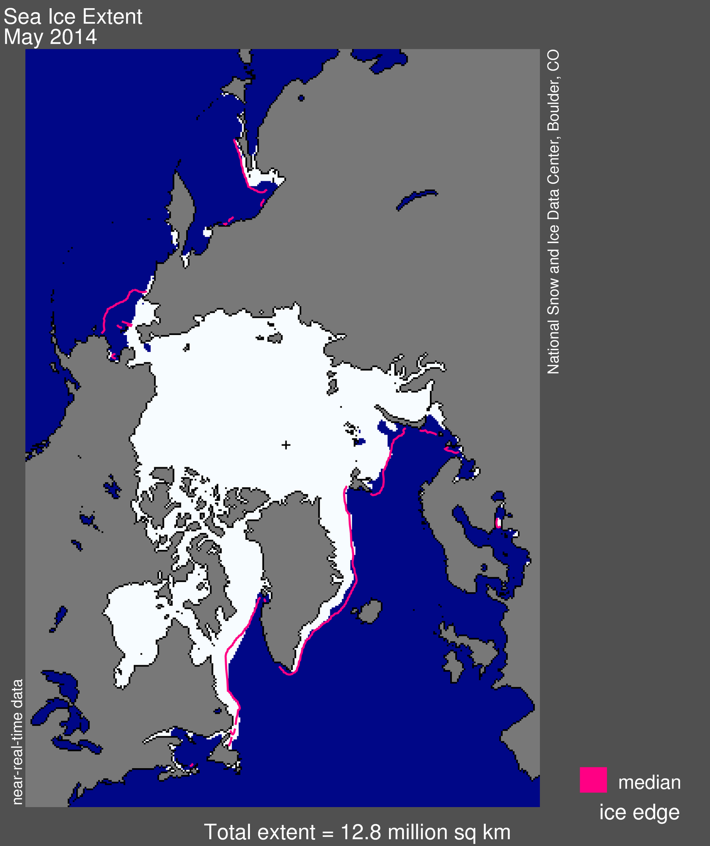
Figure 1. Arctic sea ice extent for May 2014 was 12.78 million square kilometers (4.93 million square miles). The magenta line shows the 1981 to 2010 median extent for that month. The black cross indicates the geographic North Pole. Sea Ice Index data. About the data
Credit: National Snow and Ice Data Center
High-resolution image
Arctic sea ice extent for May averaged 12.78 million square kilometers (4.93 million square miles). This is 610,000 square kilometers (235,500 square miles) below the 1981 to 2010 average for the month. May 2014 is now the third lowest May extent in the satellite record.
Ice extent was lower than average in the Barents and Bering seas. While not visible in the monthly average extent plot, the evolution of the sea ice through the month of May is characterized by the opening of several polynyas along the coast of Siberia, northern Baffin Bay, and along the coast of Hudson Bay. Nevertheless, satellites detected high sea ice concentrations over the Arctic as a whole. This contrasts with 2006, 2007, and 2012 when broad areas of low-concentration ice were observed.
As the melt season is underway in the Arctic, freeze up is in progress in the Antarctic. Sea ice extent for May averaged 12.03 million square kilometers (4.64 million square miles). This is 1.24 million square kilometers (478,800 square miles) above the 1981 to 2010 average for the month. Antarctic sea ice for May 2014 currently ranks as the highest May extent in the satellite record.
Conditions in context
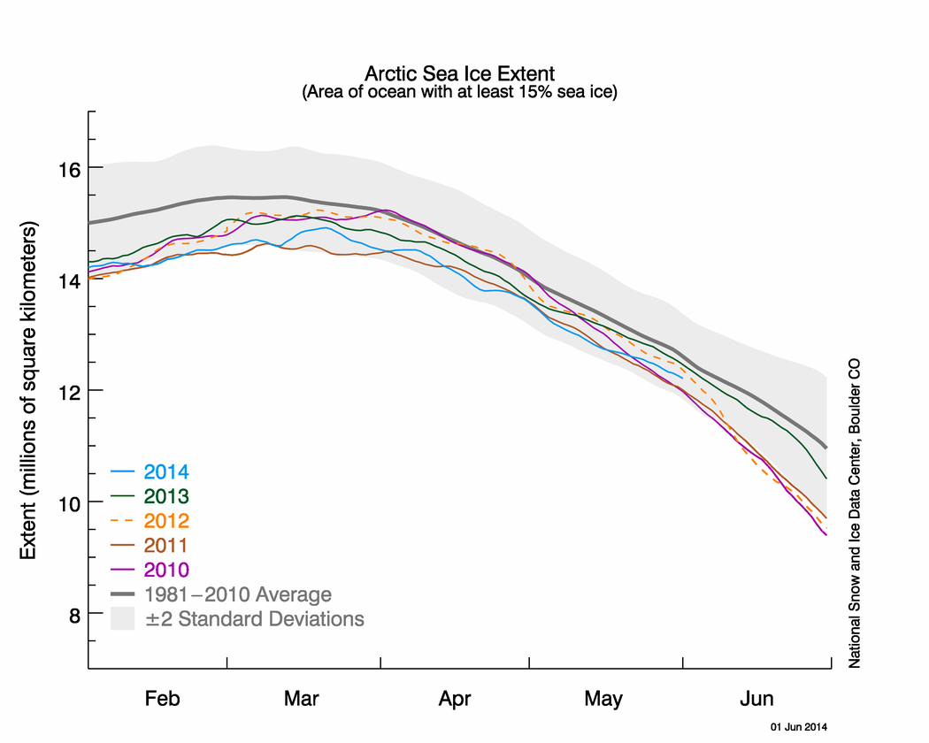
Figure 2. The graph above shows Arctic sea ice extent as of June 1, 2014, along with daily ice extent data for four previous years. 2014 is shown in blue, 2013 in green, 2012 in orange, 2011 in brown, and 2010 in purple. The 1981 to 2010 average is in dark gray. Sea Ice Index data.
Credit: National Snow and Ice Data Center
High-resolution image
May ice extent for the Arctic declined at a fairly steady rate. Sea ice retreated most rapidly in the northern Bering and southern Chukchi seas, and in the Barents Sea where a small area south of the Franz Josef Land archipelago opened late in the month. Weather was dominated by lower-than-average sea level pressure over the Central Arctic Ocean, and higher-than-average pressure over the southern Bering Sea, Alaska, and Canada. This brought about lower-than-average temperatures in the North Greenland Sea and extended toward the poles, as assessed at the 925 hPa level (roughly 3,000 feet). In contrast, warm conditions prevailed over northern Hudson Bay and southern Alaska (2 to 5 degrees Celsius or 4 to 9 degrees Fahrenheit above the 1981 to 2010 average) and the Kara and Laptev seas (1 to 2 degrees Celsius or 2 to 4 degrees Fahrenheit above the 1981 to 2010 average).
May 2014 compared to previous years
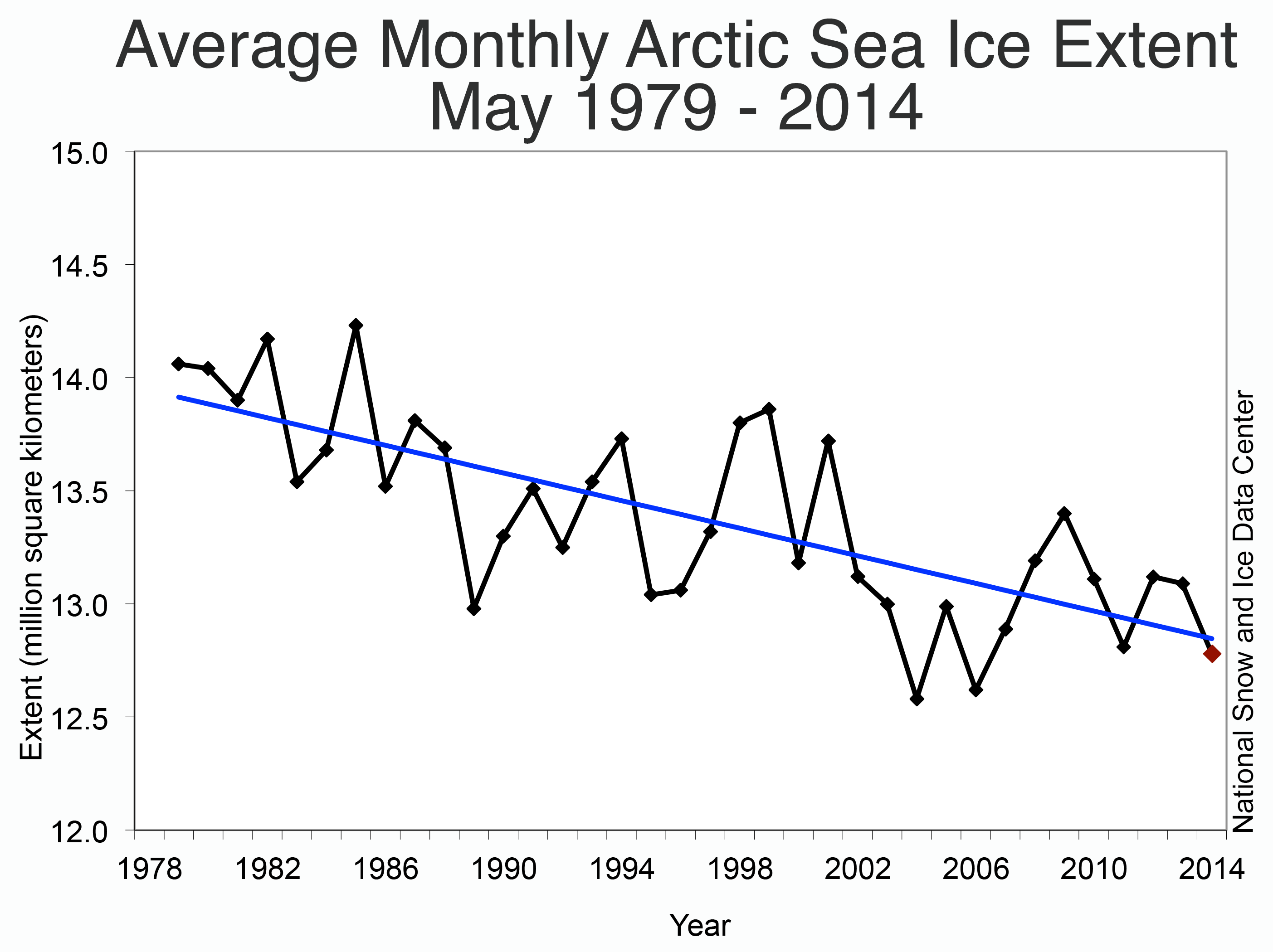
Figure 3. Monthly May ice extent for 1979 to 2014 shows a trend of -2.3% per decade relative to the 1981 to 2010 average.
Credit: National Snow and Ice Data Center
High-resolution image
Arctic sea ice extent dropped at a rate of –44,300 square kilometers (–17,100 square miles) per day, close to the average rate of –45,700 square kilometers (–17,700 square miles) per day. The monthly trend for May is now –2.3% per decade relative to the 1981 to 2010 average.
In the Antarctic, sea ice extent increased at a rate of 108,500 square kilometers (41,900 square miles) per day, very close to the average rate of 108,400 square kilometers (41,850 square miles) per day. For Antarctica, the linear rate of increase for May ice extent is 2.6% per decade relative to the 1981 to 2010 average.
Northern Hemisphere snow cover retreats rapidly
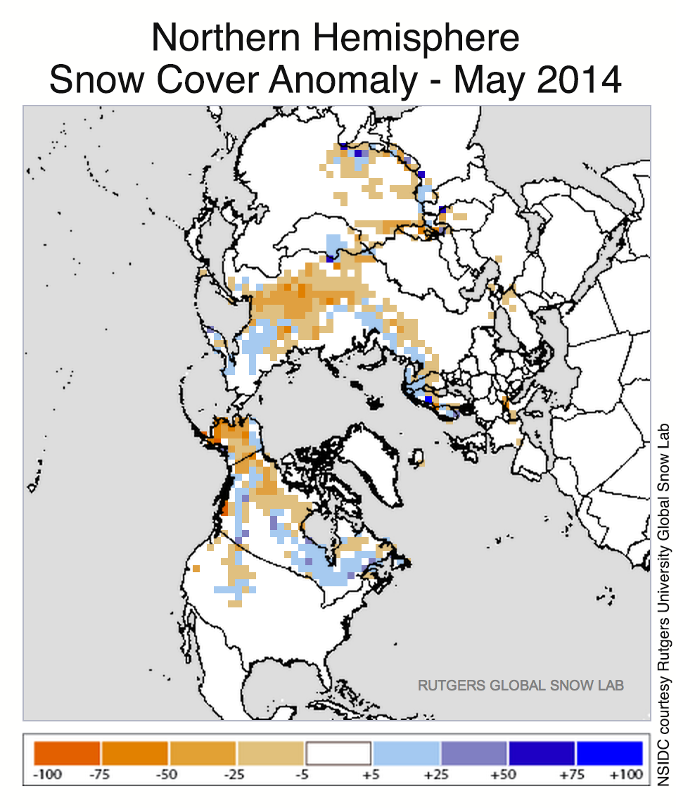
Figure 4a. This snow cover anomaly map shows the difference between snow cover for May 2014, compared with average snow cover for May from 1981 to 2010. Areas in orange and red indicate lower than usual snow cover, while regions in blue had more snow than normal.
Credit: National Snow and Ice Data Center, courtesy Rutgers University Global Snow Lab
High-resolution image
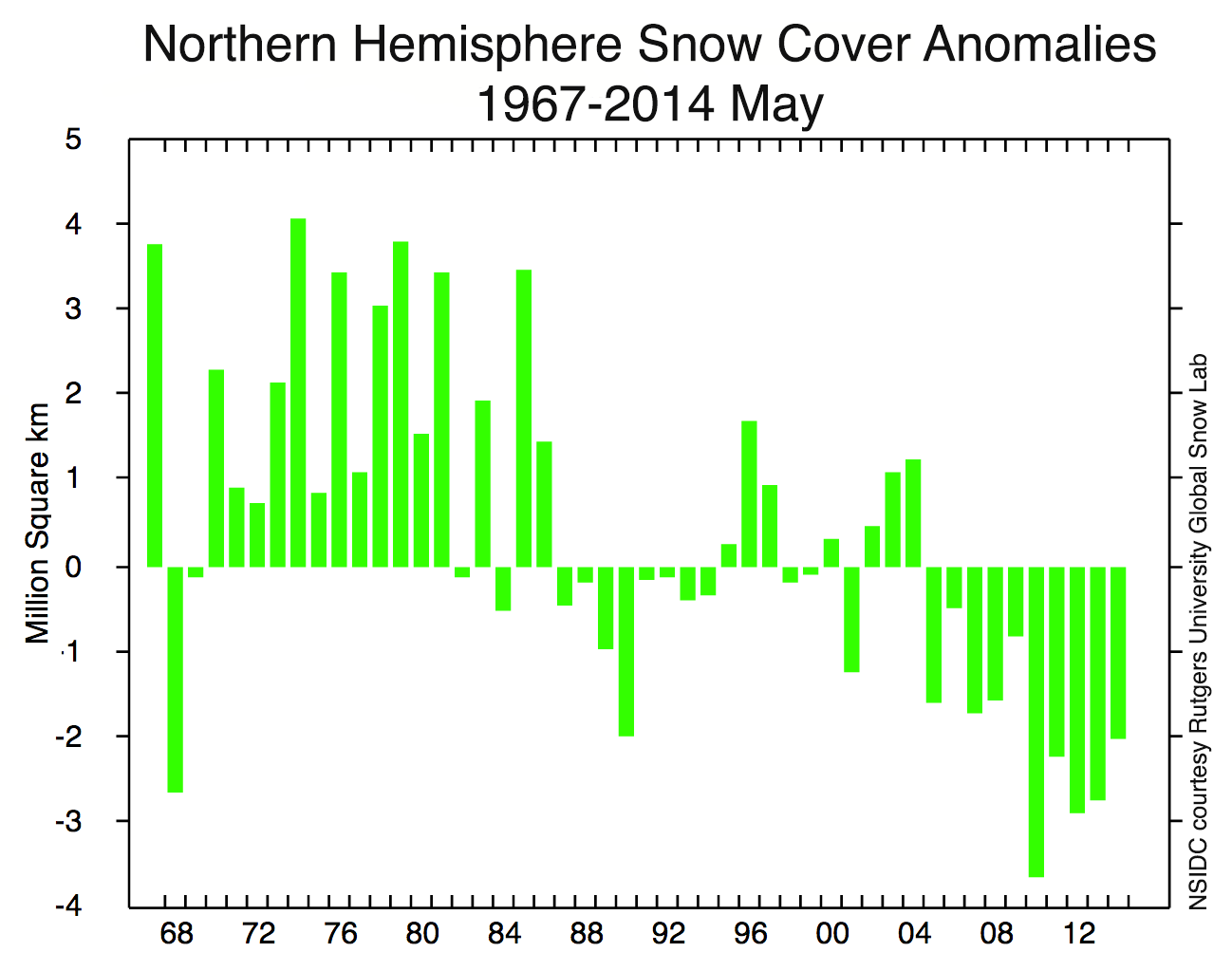
Figure 4b. This graphs shows snow cover extent anomalies in the Northern Hemisphere for May from 1967 to 2014. The anomaly is relative to the 1981 to 2010 average.
Credit: National Snow and Ice Data Center, courtesy Rutgers University Global Snow Lab
High-resolution image
After a greater-than-average snow extent in February, snow extent over the Northern Hemisphere shrank rapidly in March, April and May. The Rutgers University Global Snow Lab measured the lowest April snow extent in Eurasia in the 48-year data record. (Erratum: In an earlier version of this post, we mistakenly said that the record low April snow cover was observed in the Northern Hemisphere. We apologize for the error.) In May, snow rapidly retreated in the central Canadian Provinces in North America, and Central Asia (Kazakhstan and northwestern China), where extensive areas had above-average snow cover in February.
Snow cover in central Europe and the desert southwest of the United States were persistently below average throughout the winter and spring of 2013 to 2014. In the United States, this underscores the severe drought in the far southwest and Sierra Nevada. The rapid late spring loss in the Northern Hemisphere continues a decade-long trend toward very low snow cover early in the Arctic sea ice melt season. This resulted in warmer air over darker snow-free areas, which leads to warm air advection over the sea ice
in regions where the snow cover is anomalously low, and dry conditions in the northern boreal forests. These conditions cause increased wildfire activity and soot deposition on the sea ice and the Greenland Ice Sheet surface. High concentrations of soot on the Greenland snow pack and sea ice can contribute to ice retreat and melt.
New Arctic sea ice thickness quick look products from IceBridge, ESA CryoSat-2
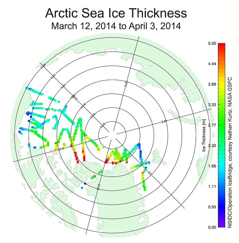
Figure 5a. Data from NASA Operation IceBridge flights over the Arctic Ocean during March and April 2014.
Credit: National Snow and Ice Data Center/NASA Operation IceBridge courtesy Nathan Kurtz
High-resolution image
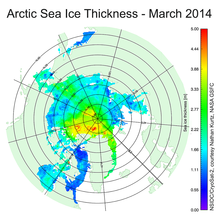
Figure 5b. This figure shows Arctic sea ice thickness for March 2014 using data from the European Space Agency’s CryoSat-2 satellite.
Credit: National Snow and Ice Data Center/NASA Operation IceBridge courtesy Nathan Kurtz
High-resolution image
The NASA IceBridge mission is an airborne campaign to augment and validate satellite measurements of sea ice and ice sheets. This spring, the NASA IceBridge program set a new record of 46 science flights, covering almost 150,000 kilometers (93,200 miles) of flight tracks from March 12, 2014 to April 3, 2014. This included flights over the western Arctic Ocean and north of Greenland to map sea ice thickness and snow depth. NSIDC has published the 2014 quick look product, in addition to a new ESA CryoSat-2 derived sea ice thickness product. Thickness estimates from both products suggest large areas within the western Beaufort Sea that are 1 to 1.5 meters (3 to 5 feet) thick. The tongue of second-year ice that extends up toward the East Siberian Sea is considerably thicker, at 2 to 3 meters (7 to 10 feet) thick. In the eastern Arctic, the ice is predominantly first-year ice, and between 1 and 1.5 meters (3 to 5 feet) thick. The thickest ice is found north of Greenland and near the pole, ranging from 3.5 to 5 meters (11 to 16 feet) thick. The timely release of thickness data from IceBridge and ESA CryoSat-2 provide a valuable resource for seasonal forecasting because they provide an estimate of the ice thickness distribution in the Arctic at the beginning of the melt season.
Forecasting needs for Arctic weather and sea ice
The National Oceanic and Atmospheric Administration (NOAA) and the U.S. Navy share a pressing need for better short-term sea ice and weather forecasts to meet their operational responsibilities. With this as a driver, the NOAA Earth Systems Research Laboratory (ESRL) hosted a workshop on Predicting Arctic Weather and Climate, and Related Impacts: Status and Requirements for Progress. The meeting was held on May 13 to 15 in Boulder, Colorado. Participants from the Office of Naval Research and the oceanographer of the Navy’s office outlined their perspective on needs for operational predictions. National Weather Service participants spoke about operational forecasting, while scientists under NOAA’s research arm along with academic scientists gave talks tailored to answering questions from forecasters. The Navy/NOAA/Coast Guard National Ice Center participated as a prime customer for better forecasting capability out of the research community. Operational needs are greatest for forecasts six to eight weeks out, where better availability of data to initialize coupled atmospheric/ocean models offers promise for improvement. Seasonal forecasts of ice melt can be improved with better ice thickness initialization fields. The predictability of the timing of freeze-up at the end of the season appears to depend upon improved sea surface temperature fields.
The NOAA Arctic Action Plan and the U.S. Navy’s Arctic Roadmap give a high-level view of how these agencies are addressing change in the Arctic.
Reference
Kurtz, N. T., Galin, N., and Studinger, M. 2014. An improved CryoSat-2 sea ice freeboard and thickness retrieval algorithm through the use of waveform fitting, The Cryosphere Discuss., 8, 721-768, doi:10.5194/tcd-8-721-2014.

