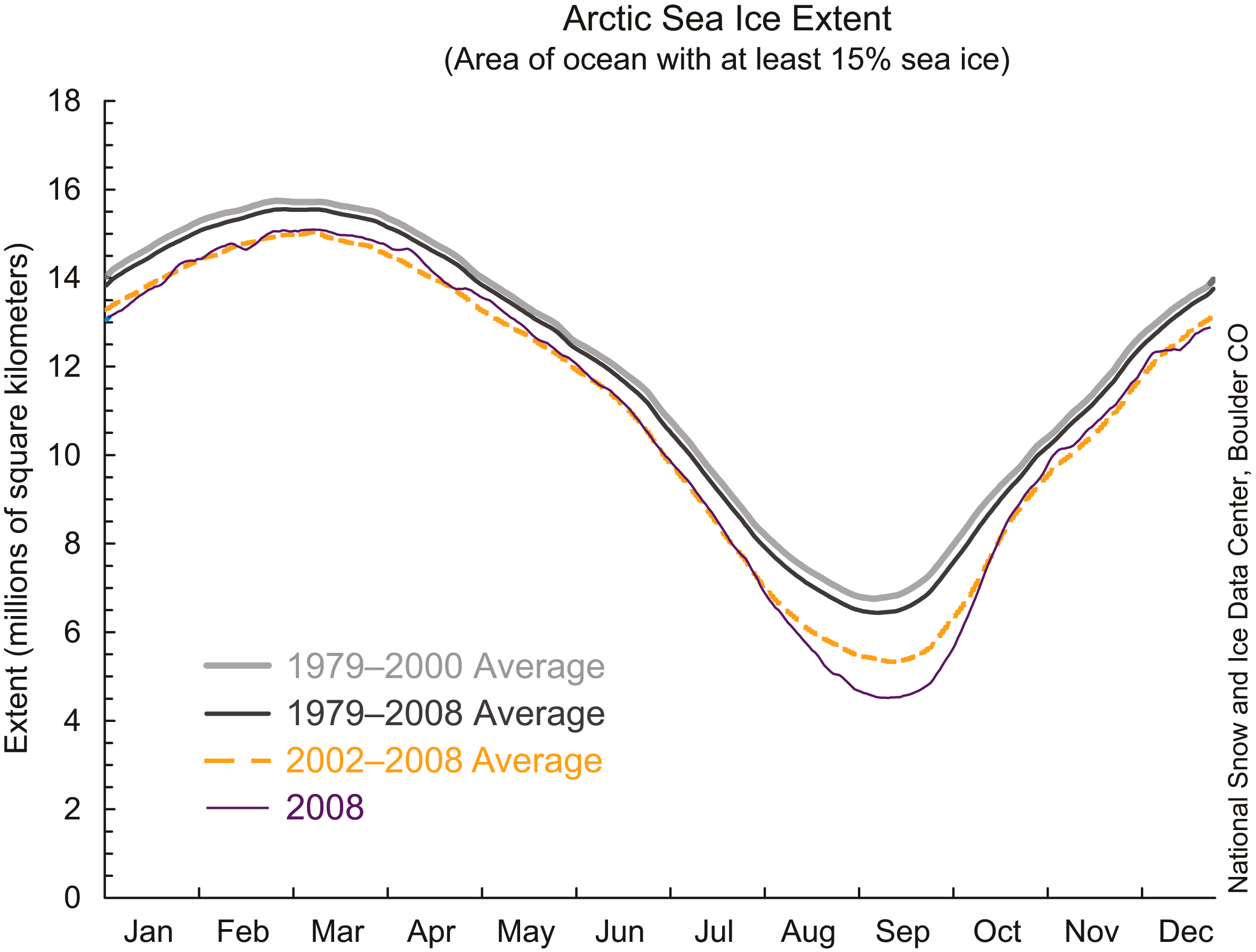
Arctic sea ice extent has begun its seasonal decline towards the September minimum. Ice extent through the winter was similar to that of recent years, but lower than the 1979 to 2000 average. More importantly, the melt season has begun with a substantial amount of thin first-year ice, which is vulnerable to summer melt.
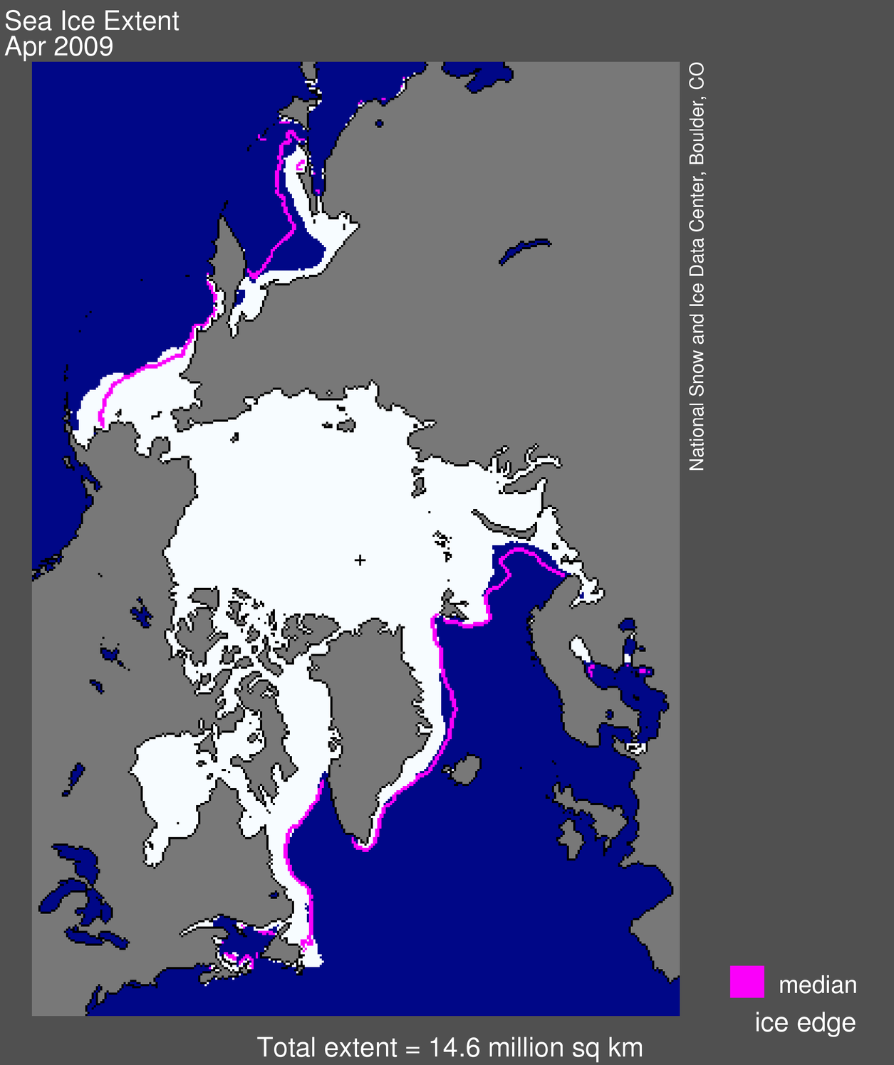
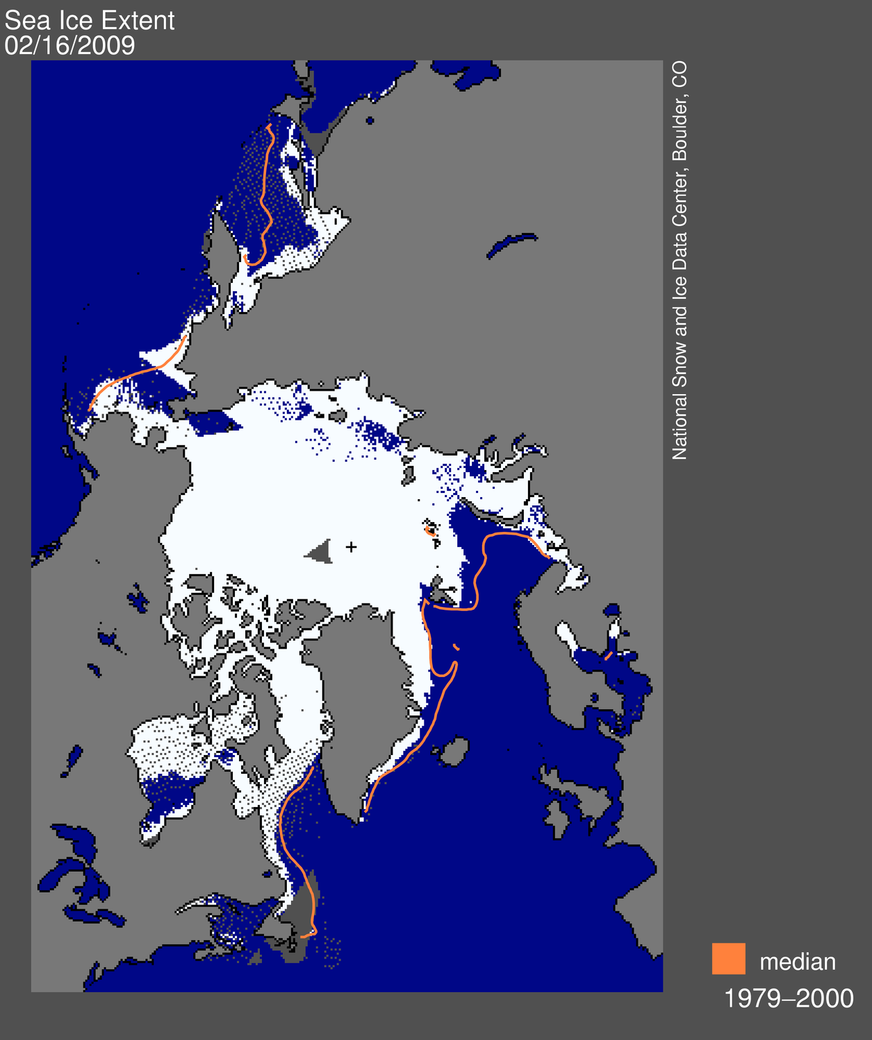
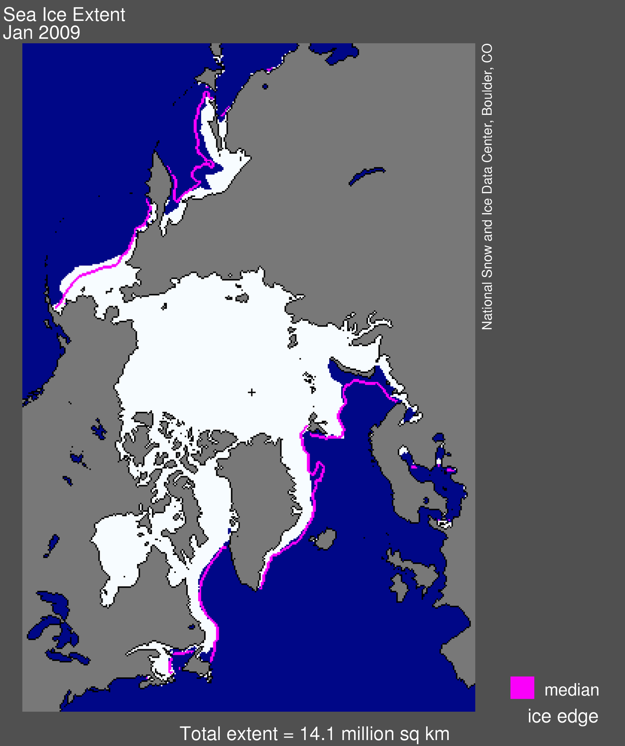
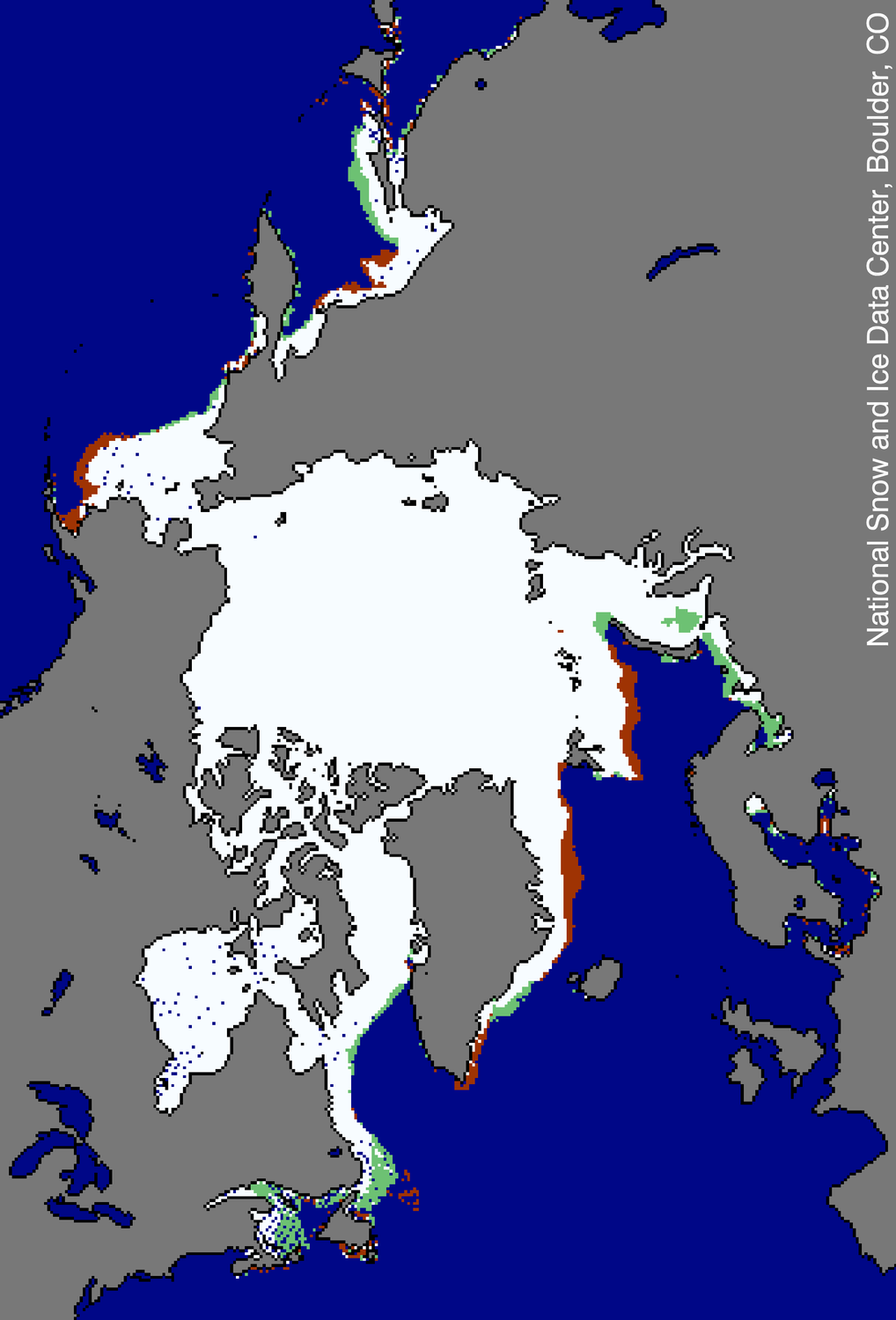
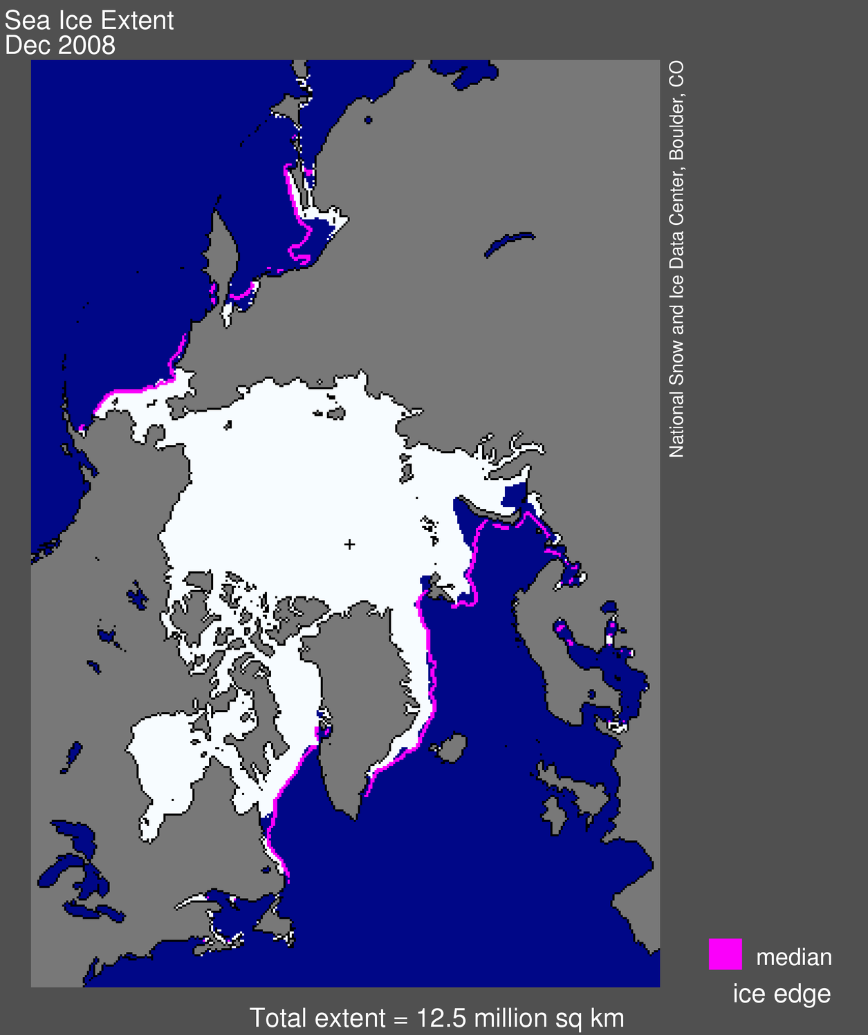
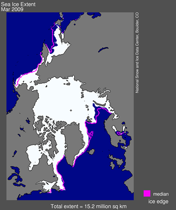 Figure 1. Arctic sea ice extent for March, 2009, was 15.16 million square kilometers (5.85 million square miles). The magenta line shows the 1979 to 2000 median extent for that month. The black cross indicates the geographic North Pole. Sea Ice Index data. About the data. —Credit: National Snow and Ice Data Center
High-resolution image
Figure 1. Arctic sea ice extent for March, 2009, was 15.16 million square kilometers (5.85 million square miles). The magenta line shows the 1979 to 2000 median extent for that month. The black cross indicates the geographic North Pole. Sea Ice Index data. About the data. —Credit: National Snow and Ice Data Center
High-resolution image
Overview of conditions
Sea ice extent averaged over the month of March 2009 was 15.16 million square kilometers (5.85 million square miles). This was 730,000 square kilometers (282,000 square miles) above the record low of 2006, but 590,000 square kilometers (228,000 square miles) below the 1979 to 2000 average.
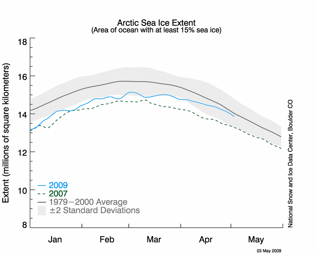
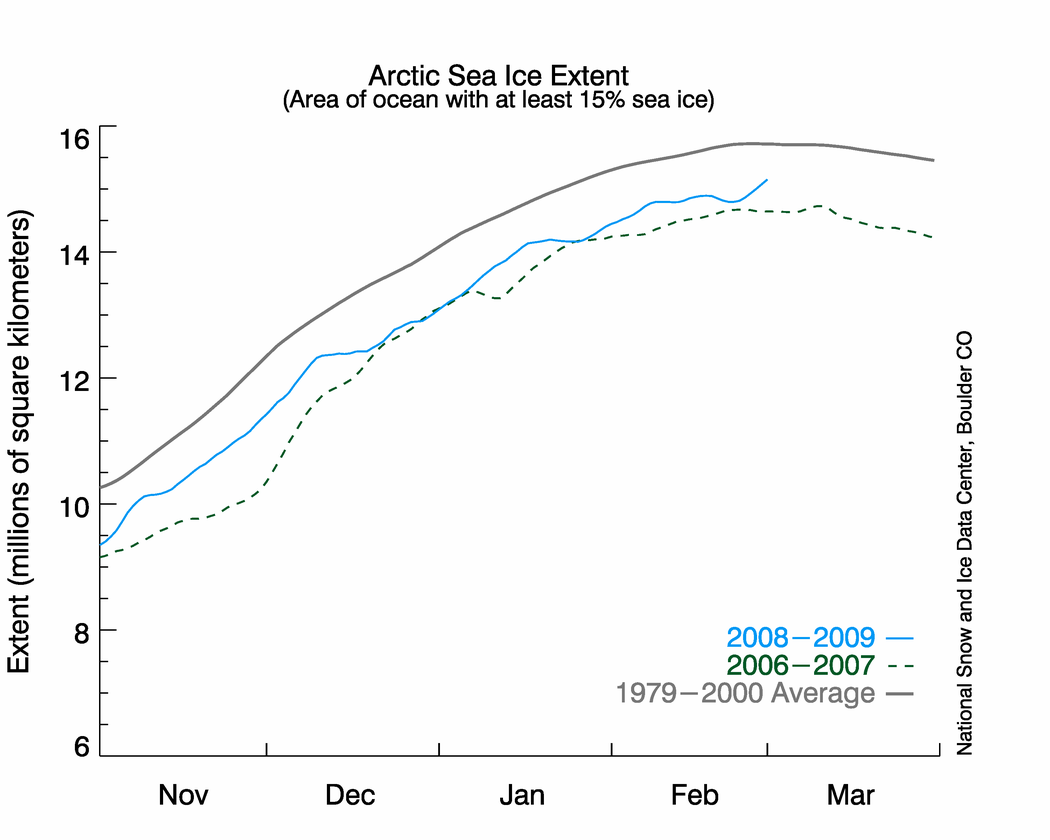
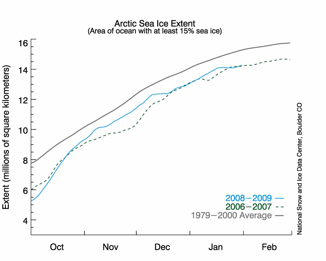
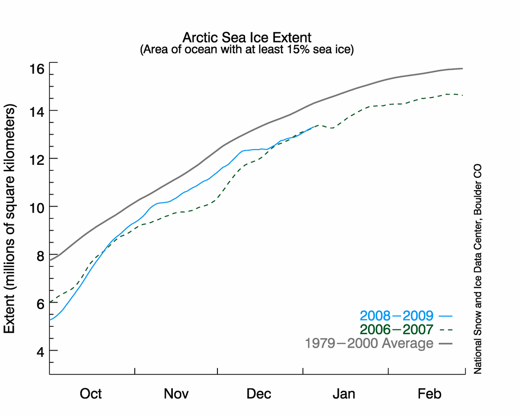
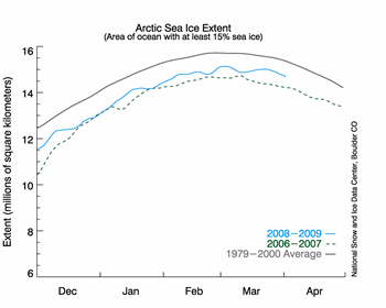 Figure 2. The graph above shows daily sea ice extent. The solid blue line indicates 2008 to 2009; the dashed green line shows 2006 to 2007 (the record-low summer minimum occurred in 2007); and the solid gray line indicates average extent from 1979 to 2000. Sea Ice Index data.—Credit: National Snow and Ice Data
Center
High-resolution image
Conditions in context
At the end of last summer’s melt season, extensive areas of open
water froze up quickly, once air temperatures cooled in
the fall. By February 28, ice extent had reached its annual maximum.
Although the maximum ice extent occurred slightly earlier than usual, ice extent remained close to the maximum level through much
of March.
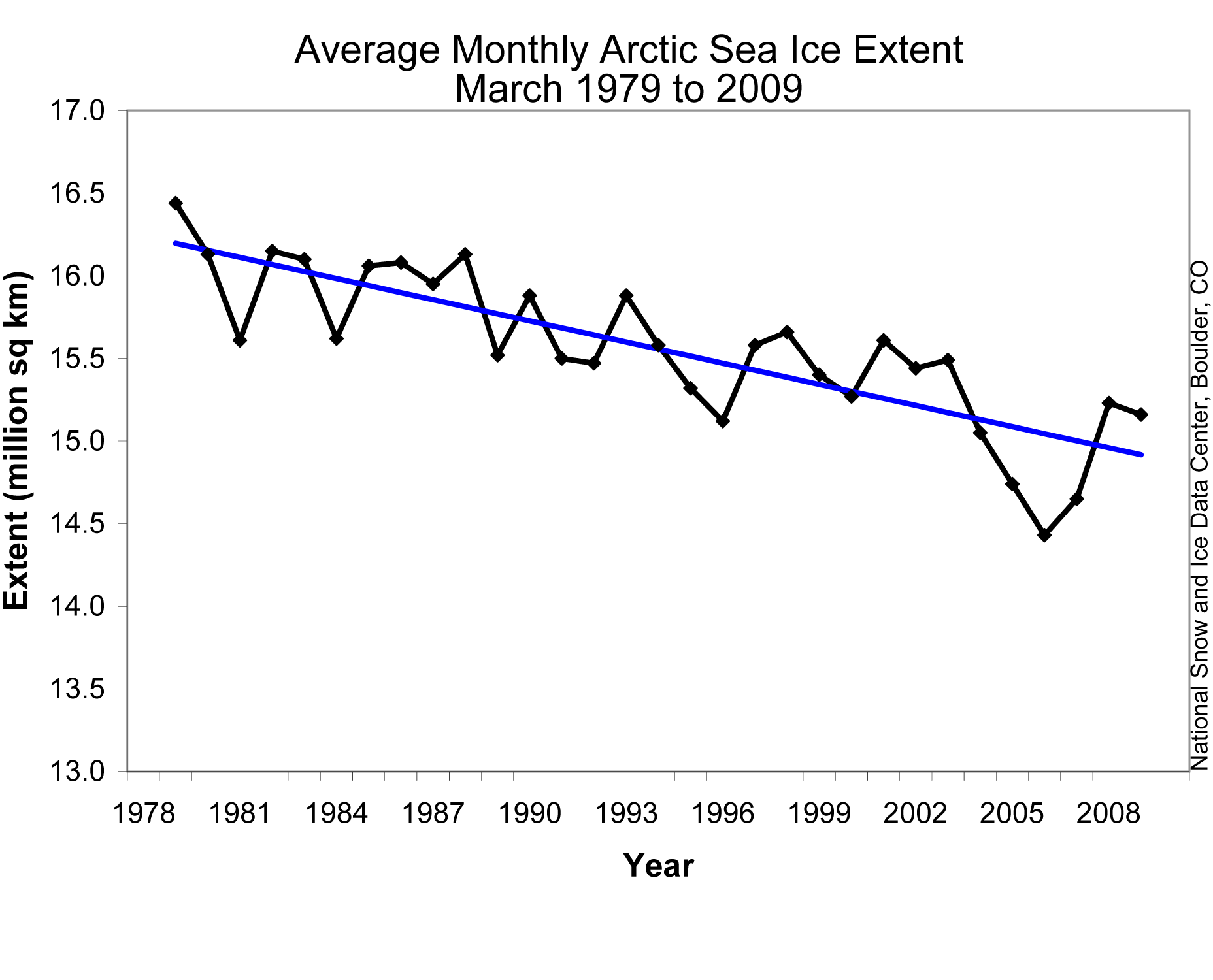
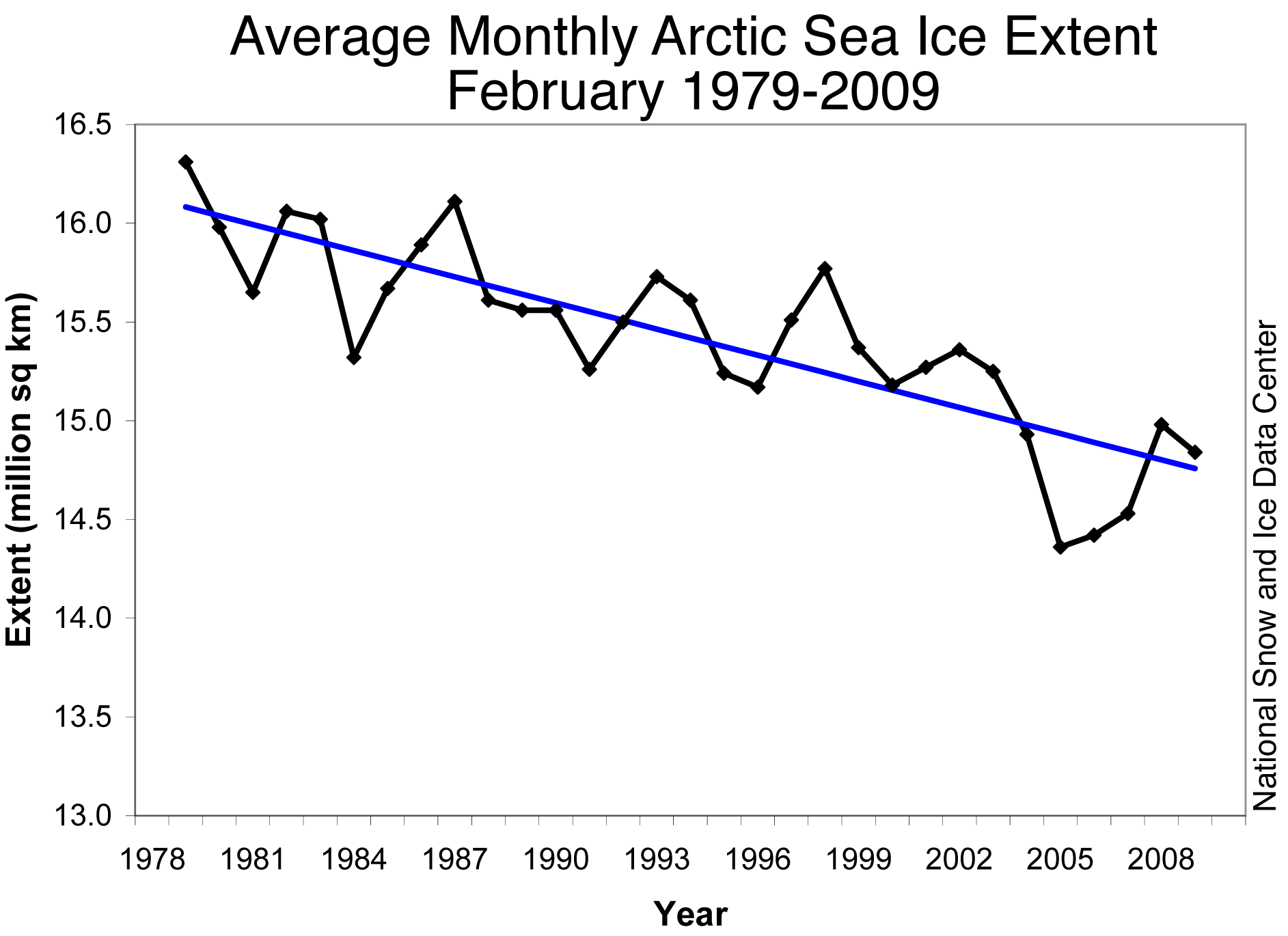
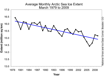 Figure 3. Monthly March ice extent for 1979 to 2009 shows a decline of 2.7% per decade.—Credit: National Snow and Ice Data Center
High-resolution image
Figure 3. Monthly March ice extent for 1979 to 2009 shows a decline of 2.7% per decade.—Credit: National Snow and Ice Data Center
High-resolution image
March 2009 compared to past Marches
Including March 2009, the past six years have all had ice extent substantially lower than normal. The linear trend indicates that for the month of March, ice extent is declining by 2.7% per decade, an average of 43,000 square kilometers (16,000 square miles) of ice per year.
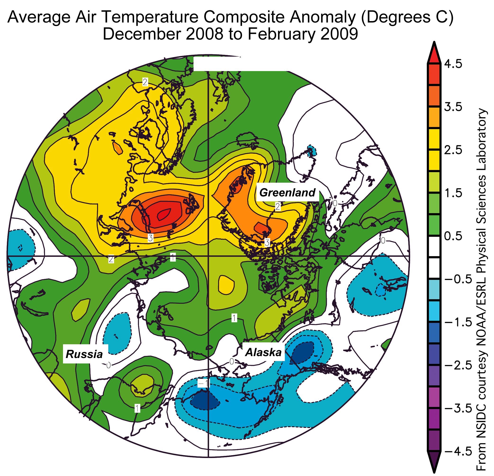
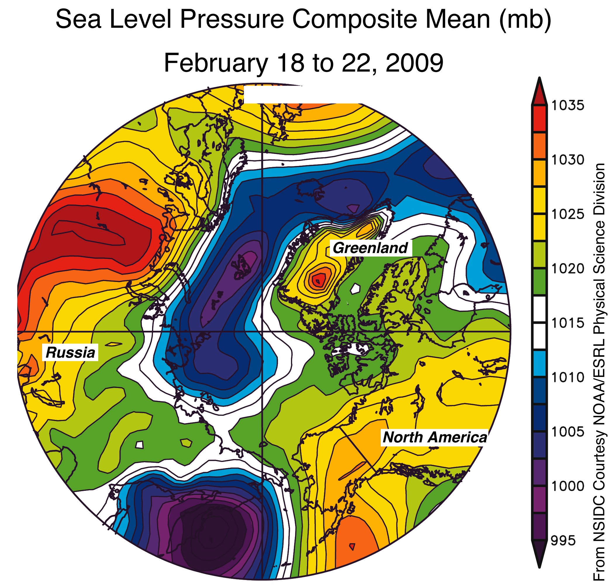
 Figure 4. The map of air temperature anomalies for winter 2008 to 2009 at the 925 millibar level (roughly 1,000 meters [3,000 feet] above the surface) shows warmer-than-usual conditions over much of the Arctic Ocean. Areas in orange and red correspond to strong positive (warm) anomalies. Areas in blue correspond to negative (cool) anomalies.—Credit: National Snow and Ice Data Center courtesy NOAA/ESRL Physical Sciences Laboratory
High-resolution image
Figure 4. The map of air temperature anomalies for winter 2008 to 2009 at the 925 millibar level (roughly 1,000 meters [3,000 feet] above the surface) shows warmer-than-usual conditions over much of the Arctic Ocean. Areas in orange and red correspond to strong positive (warm) anomalies. Areas in blue correspond to negative (cool) anomalies.—Credit: National Snow and Ice Data Center courtesy NOAA/ESRL Physical Sciences Laboratory
High-resolution image
Arctic winter warmer than average
Overall, it was a fairly warm winter in the Arctic. Air temperatures over the Arctic Ocean were an average of 1 to 2 degrees Celsius (1.8 to 3.6 degrees Fahrenheit) above normal, with notable regional variations. The Barents Sea region was over 4 degrees Celsius (7.2 degrees Fahrenheit) warmer than average this winter. This warmth probably stemmed from unusually low sea ice extent in the region throughout much of the winter, which allowed the ocean to pump heat into the atmosphere. The Bering Sea, in contrast, experienced a cool winter, with temperatures 1 to 2 degrees Celsius (1.8 to 3.6 degrees Fahrenheit) below average. The cooler conditions were consistent with the above-average sea ice extent in the Bering Sea through much of the winter.
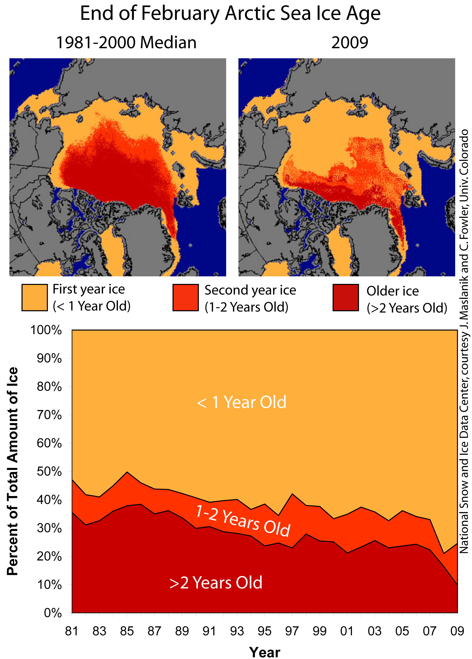
 Figure 5. These images show declining sea ice age, which indicates a thinning Arctic sea ice cover more vulnerable to melting in summer. Ice older than two years now accounts for less than 10% of the ice cover.—Credit: From the National Snow and Ice Data Center, courtesy J. Maslanik and C. Fowler, University of Colorado
High-resolution image
Figure 5. These images show declining sea ice age, which indicates a thinning Arctic sea ice cover more vulnerable to melting in summer. Ice older than two years now accounts for less than 10% of the ice cover.—Credit: From the National Snow and Ice Data Center, courtesy J. Maslanik and C. Fowler, University of Colorado
High-resolution image
Sea ice young and thin as melt season begins
How vulnerable is the ice cover as we go into the summer melt season? To answer this question, scientists also need information about ice thickness. Indications of winter ice thickness, commonly derived from ice age estimates, reveal that the ice is thinner than average, suggesting that it is more susceptible to melting away during the coming summer.
As the melt season begins, the Arctic Ocean is covered mostly by first-year ice, which formed this winter, and second-year ice, which formed during the winter of 2007 to 2008. First-year ice in particular is thinner and more prone to melting away than thicker, older, multi-year ice. This year, ice older than two years accounted for less than 10% of the ice cover at the end of February. From 1981 through 2000, such older ice made up an average of 30% of the total sea ice cover at this time of the year.
While ice older than two years reached record lows, the fraction of second-year sea ice increased compared to last winter. Some of this second-year ice will survive the summer melt season to replenish the Arctic’s store of older ice; however, in recent years less young ice has made it through the summer. To restore the amount of older ice to pre-2000 levels, large amounts of this young ice would need to endure through summer for several years in a row.
But conditions may not always favor the survival of second-year and older ice. Each winter, winds and ocean currents move some sea ice out of the Arctic ocean. This winter, some second-year ice survived the 2008 melt season only to be pushed out of the Arctic by strong winter winds. Based on sea ice age data from Jim Maslanik and Chuck Fowler at the University of Colorado, since the end of September 2008, 390,000 square kilometers (150,000 square miles) of second-year ice and 190,000 square kilometers (73,000 square miles) of older (more than two years old) ice moved out of the Arctic. View
animation (1.1 MB).
References:
Maslanik J. A., C. Fowler, J. Stroeve, S. Drobot, J. Zwally, D. Yi, W. Emery. 2007. A younger, thinner Arctic ice cover: Increased potential for rapid, extensive sea-ice loss. Geophysical Research Letters, 34, L24501, doi:10.1029/2007GL032043.
Fowler, C., W. J. Emery, and J. Maslanik. 2004. Satellite-derived evolution of Arctic sea ice age: October 1978 to March 2003. IEEE Geosci. Remote Sensing Letters, 1(2), 71–74, doi:10.1109/LGRS.2004.824741.
For previous analysis, please see the drop-down menu under Archives in the right navigation at the top of this page.
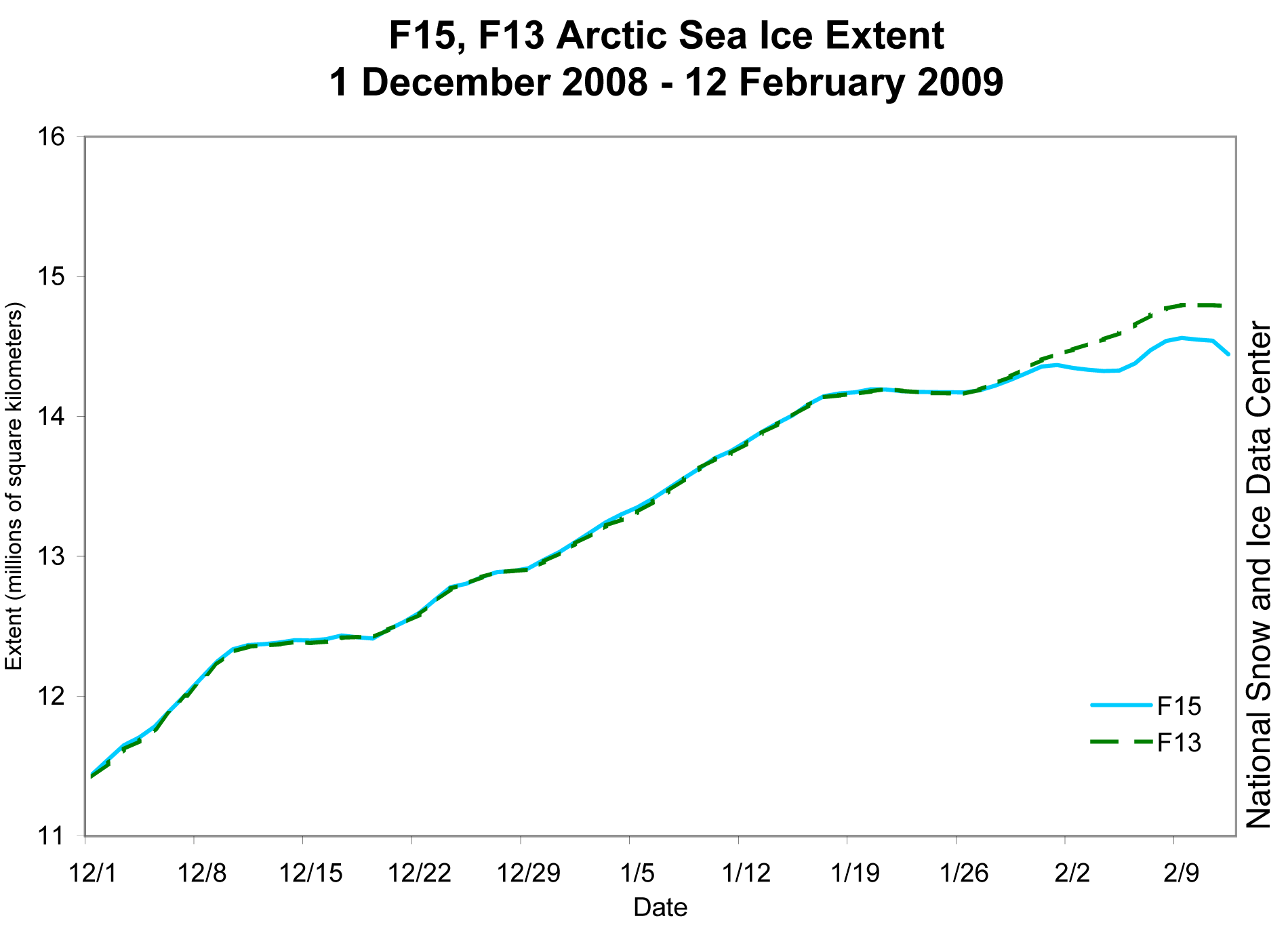
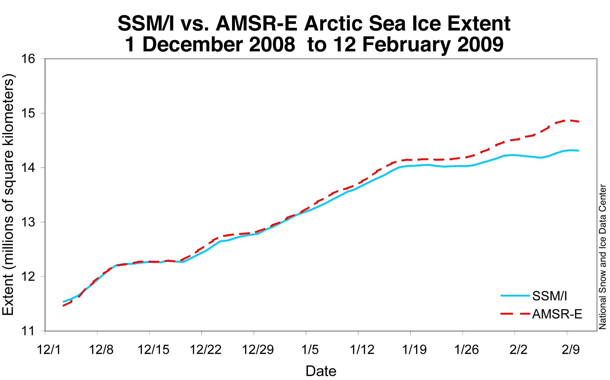
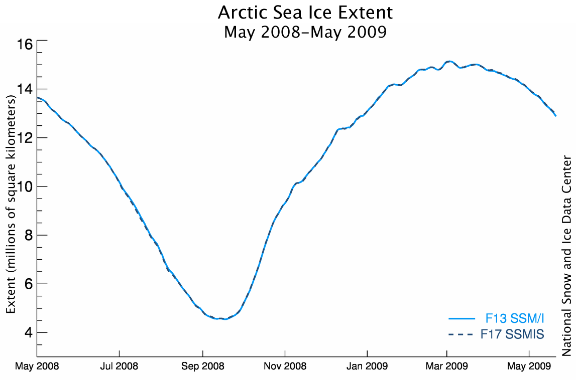 Figure 1. NSIDC now has more than a year of data from the Special Sensor Microwave Imager/Sounder (SSMIS) sensor on the DMSP F17 satellite, which has been intercalibrated with data from the F13 satellite. Note the close correspondence between the two data records. The average absolute daily difference was approximately 28,000 square kilometers (11,000 square miles). Sea Ice Index data. About the data. —Credit: National Snow and Ice Data Center