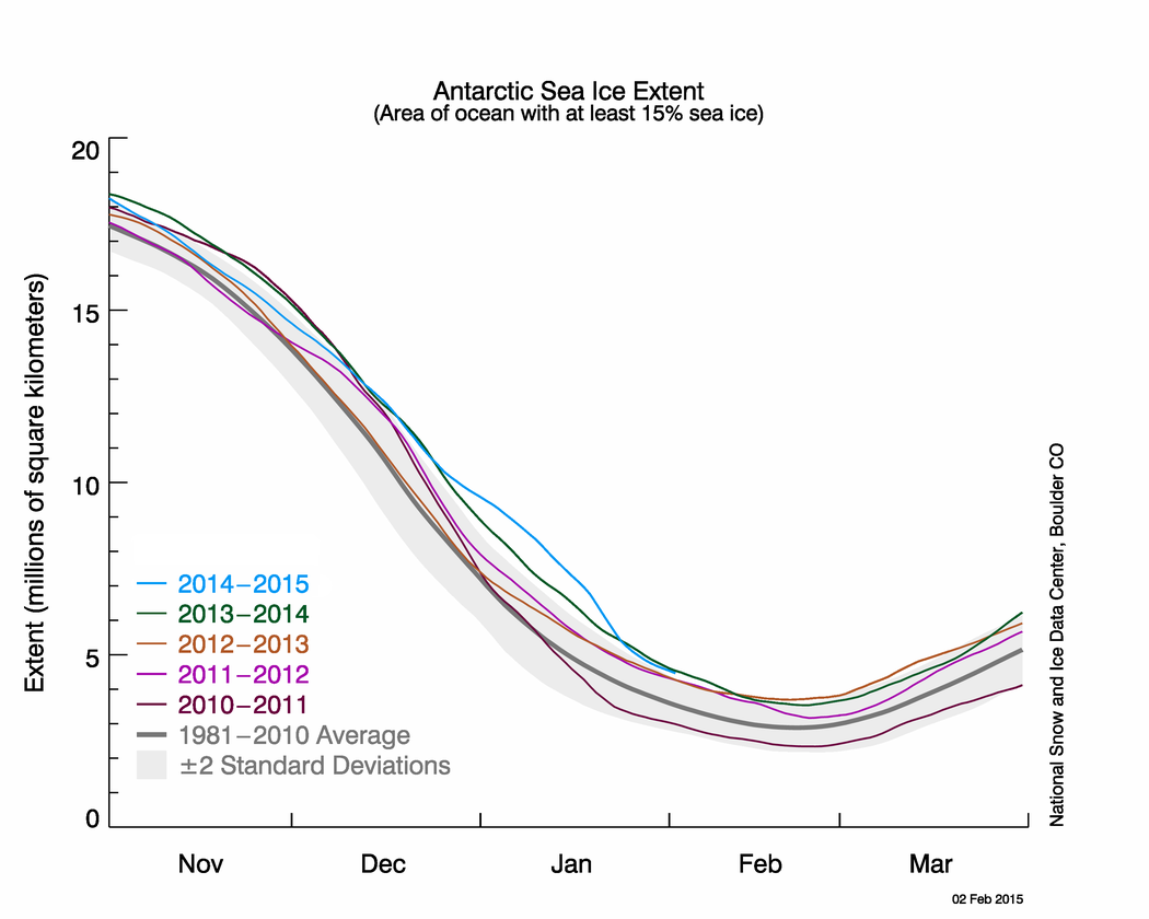
After reaching its seasonal maximum on February 25, the beginning of the melt season was interrupted by late-season periods of ice growth, largely in the Bering Sea, Davis Strait and around Labrador. Near the end of March, extent rose to within about 83,000 square kilometers (32,000 square miles) of the February 25 value. The monthly average Arctic sea ice extent for March was the lowest in the satellite record.

Overview of conditions

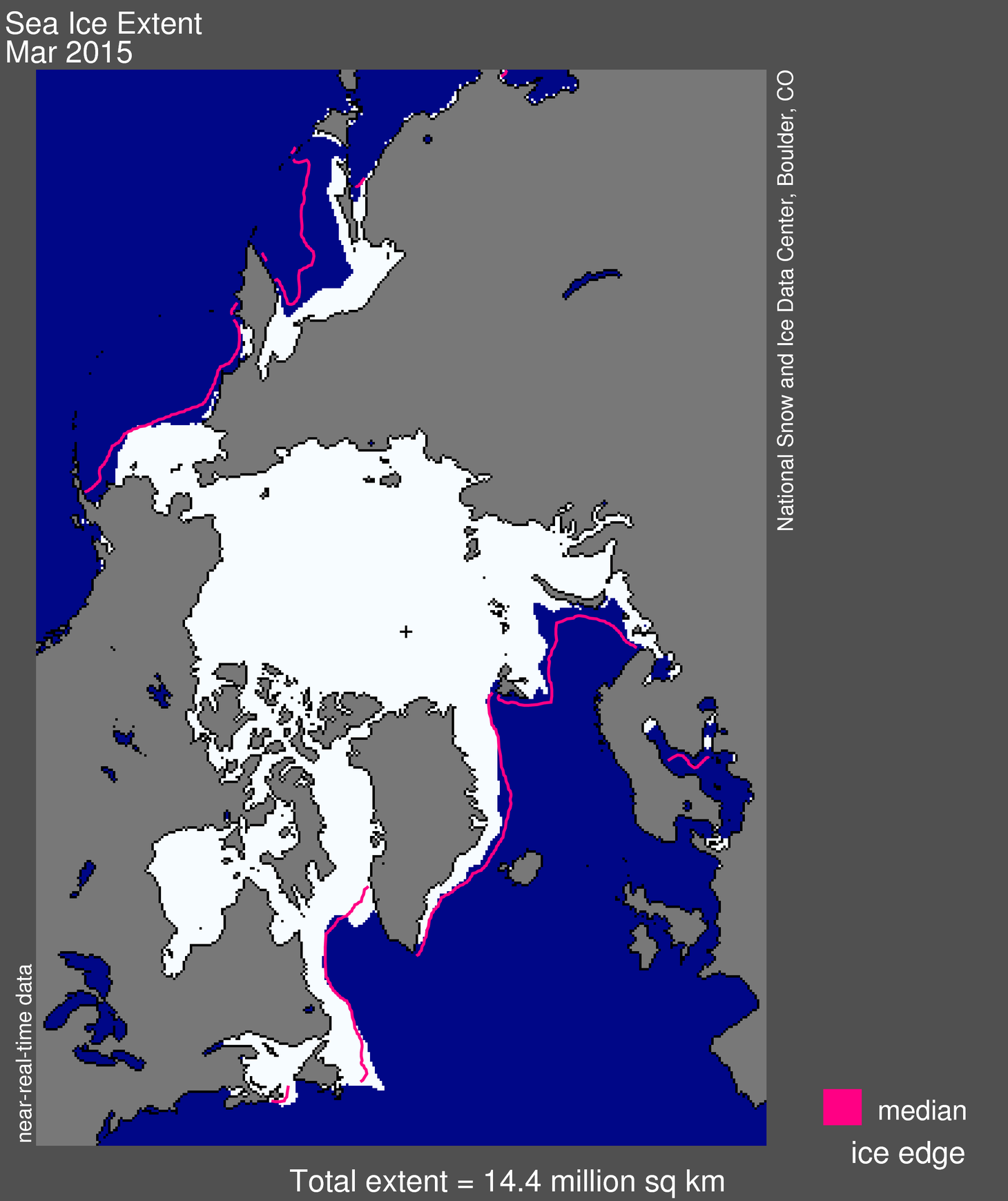
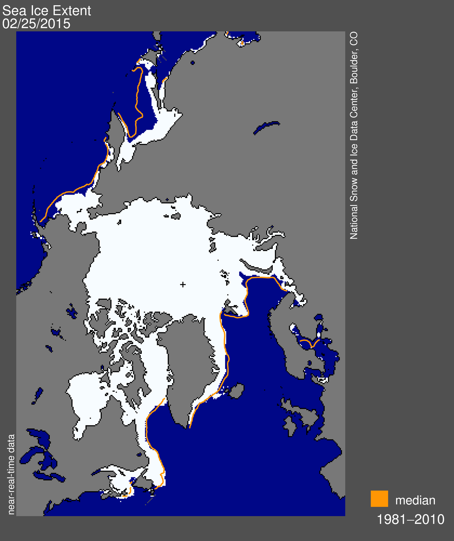
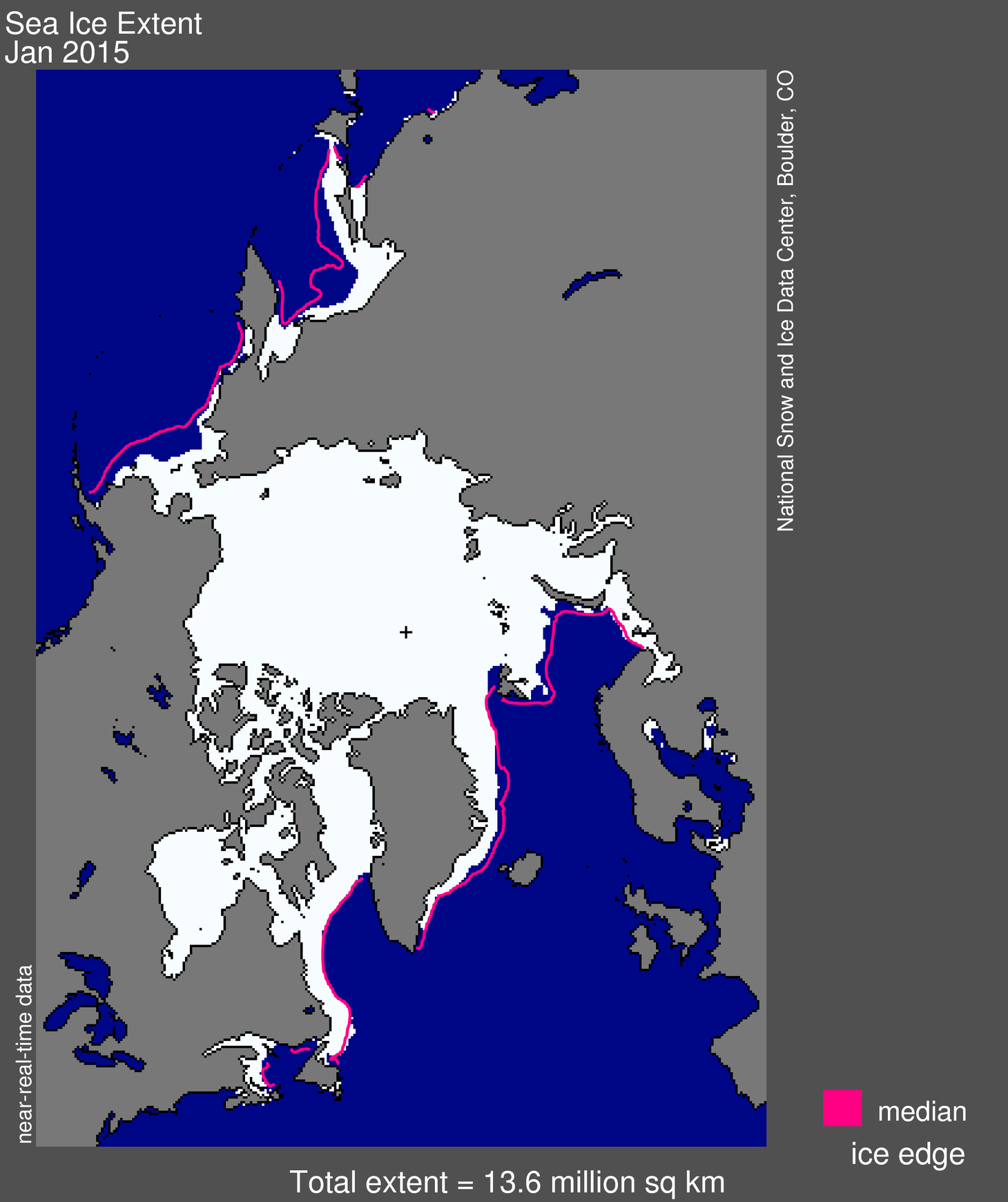
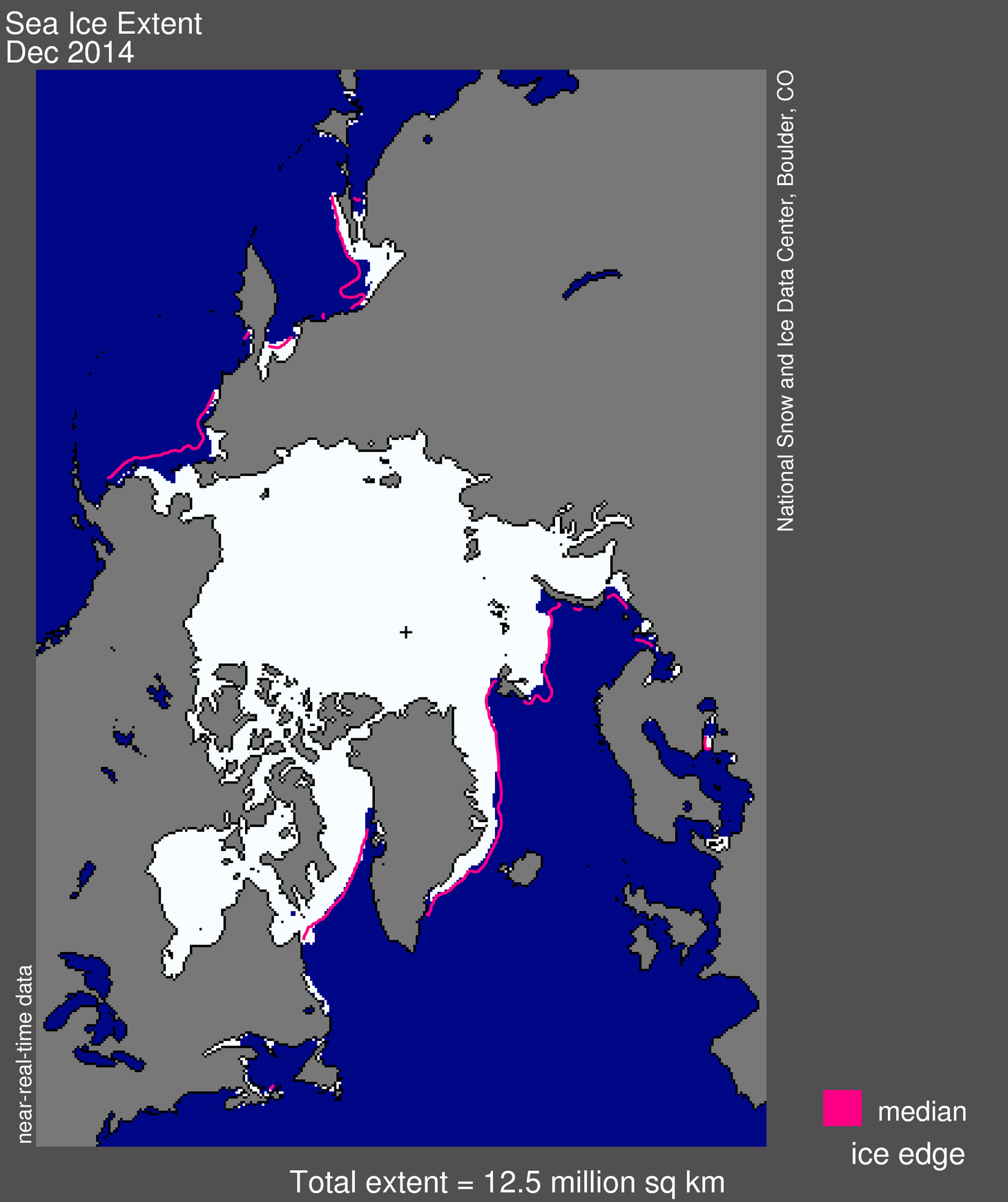
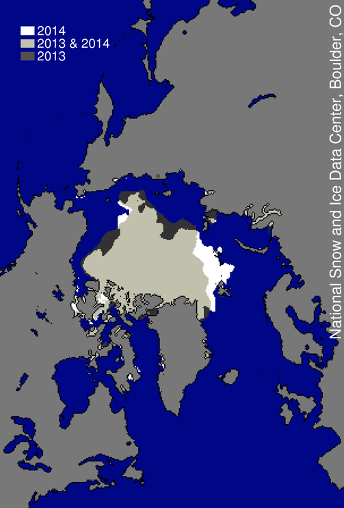
Figure 1. Arctic sea ice extent for March 2015 was 14.39 million square kilometers (5.56 million square miles). The magenta line shows the 1981 to 2010 median extent for that month. The black cross indicates the geographic North Pole. Sea Ice Index data. About the data

Credit: National Snow and Ice Data Center
High-resolution image

Arctic sea ice extent for March 2015 averaged 14.39 million square kilometers (5.56 million square miles). This is the lowest March ice extent in the satellite record. It is 1.13 million square kilometers (436,000 square miles) below the 1981 to 2010 long-term average of 15.52 million square kilometers (6.00 million square miles). It is also 60,000 square kilometers (23,000 square miles) below the previous record low for the month observed in 2006.

Conditions in context

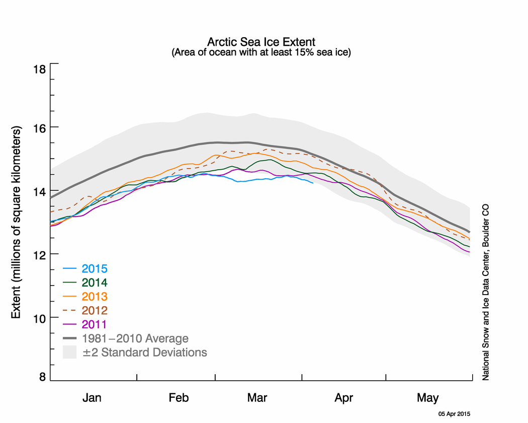
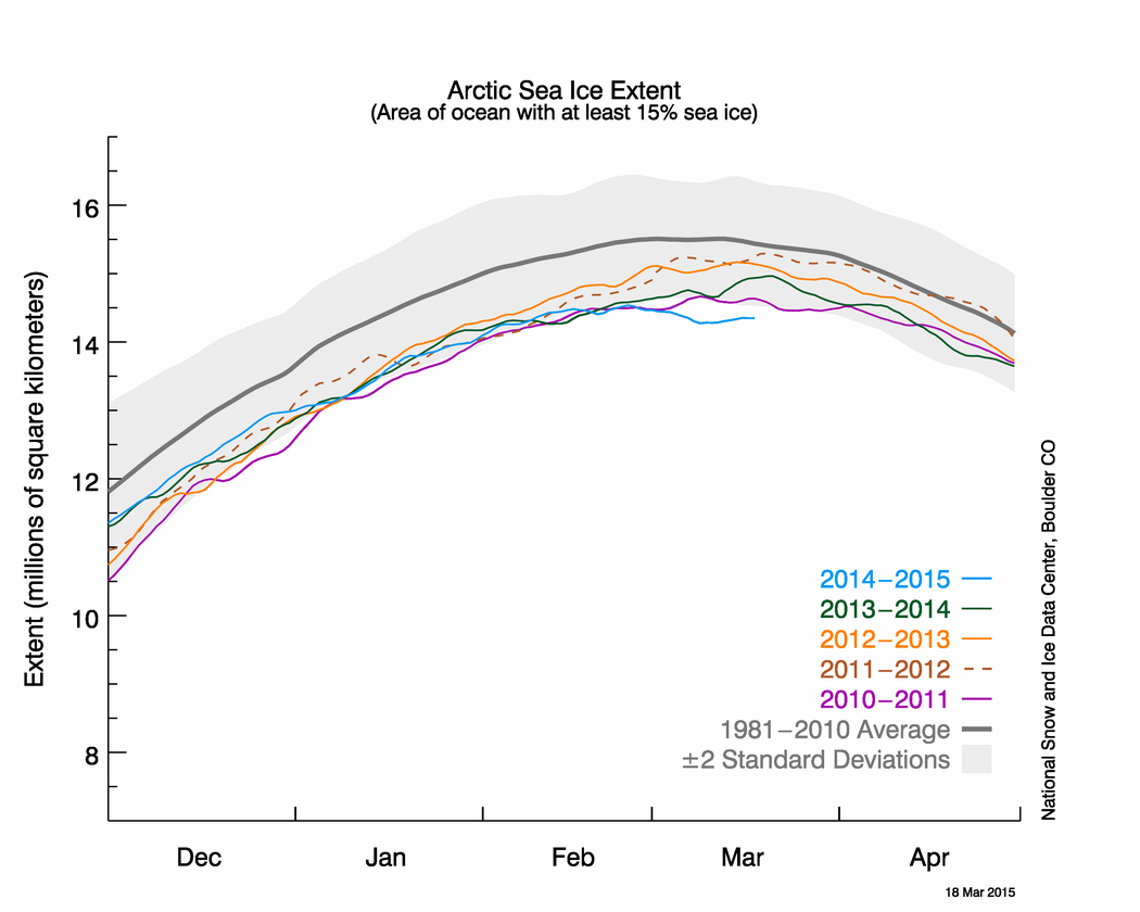
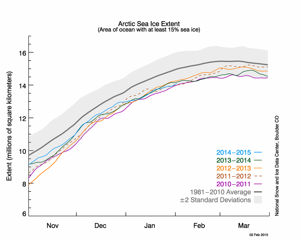
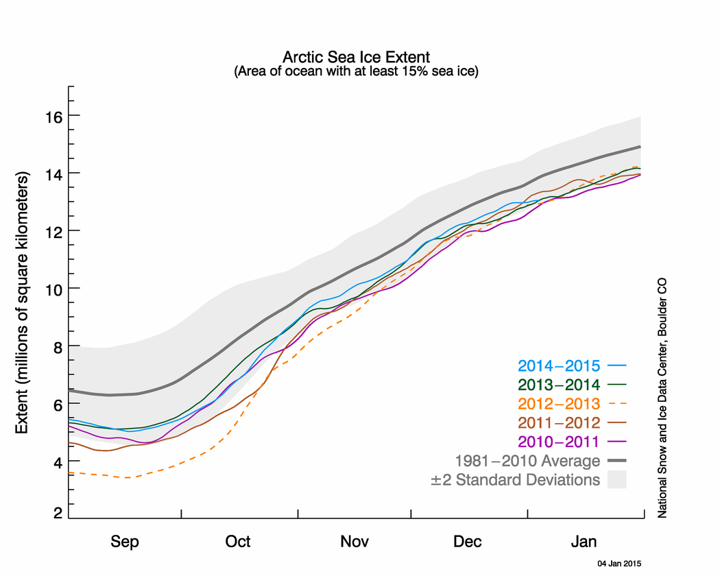
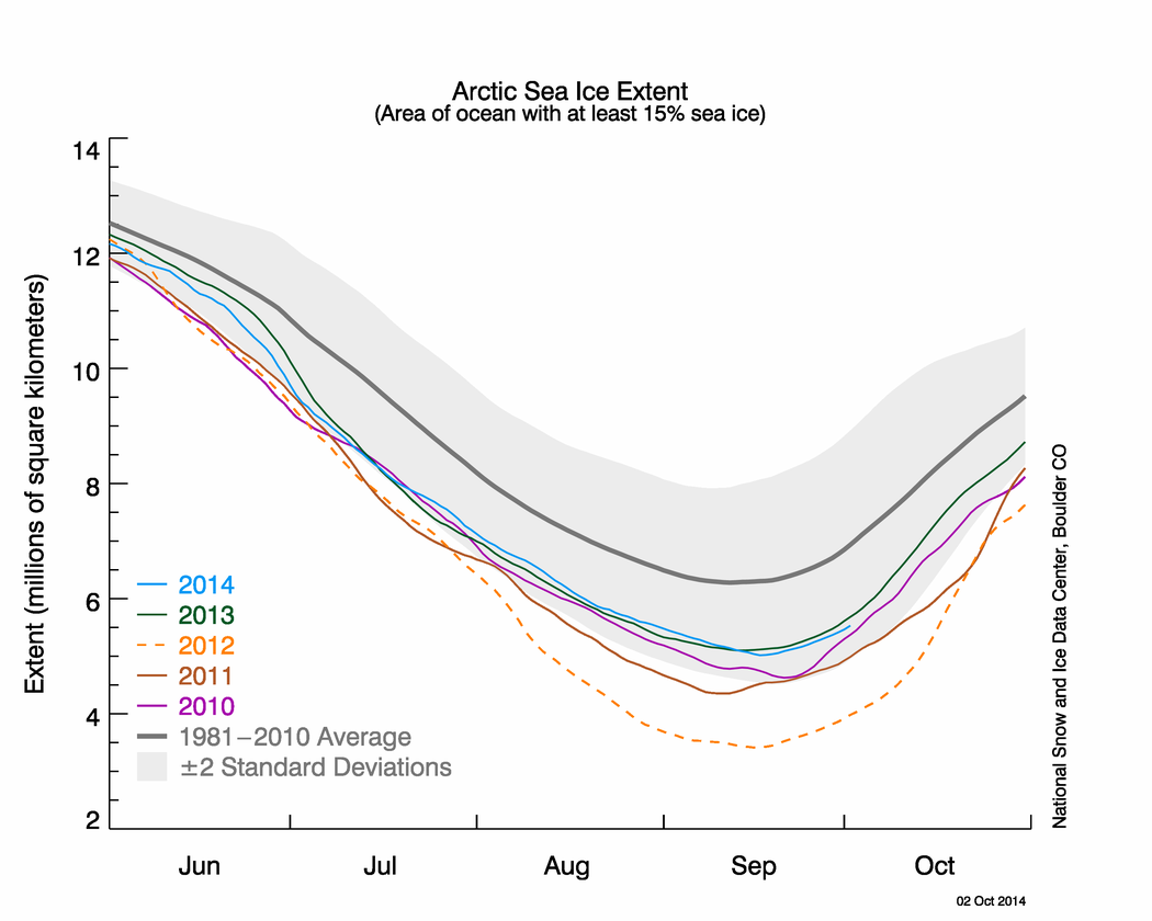
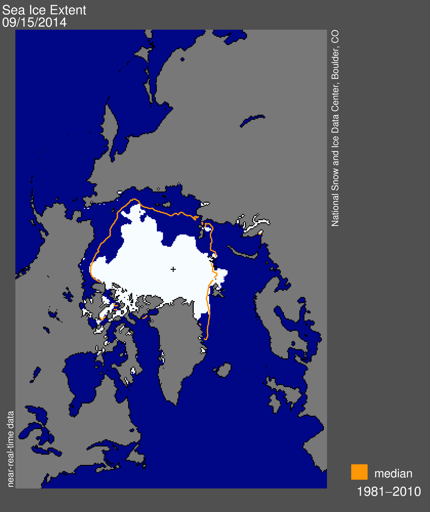
Figure 2. The graph above shows Arctic sea ice extent as of April 5, 2015, along with daily ice extent data for four previous years. 2015 is shown in blue, 2014 in green, 2013 in orange, 2012 in brown, and 2011 in purple. The 1981 to 2010 average is in dark gray. The gray area around the average line shows the two standard deviation range of the data. Sea Ice Index data.

Credit: National Snow and Ice Data Center
High-resolution image

The change in total Arctic sea ice extent for March is typically quite small. It tends to increase slightly during the first part of the month, reach the seasonal maximum, and then decline over the remainder of the month. Following the seasonal maximum recorded on February 25, this year instead saw a small decline over the first part of March, and then an increase, due largely to periods of late ice growth in the Bering Sea, Davis Strait and around Labrador. On March 26, extent had climbed to within 83,000 square kilometers (32,000 square miles) of the seasonal maximum recorded on February 25. Despite this late-season ice growth, analysts at the Alaska Ice Program report in their April 3 post that ice in the Bering Sea was very broken up.

March 2015 compared to previous years

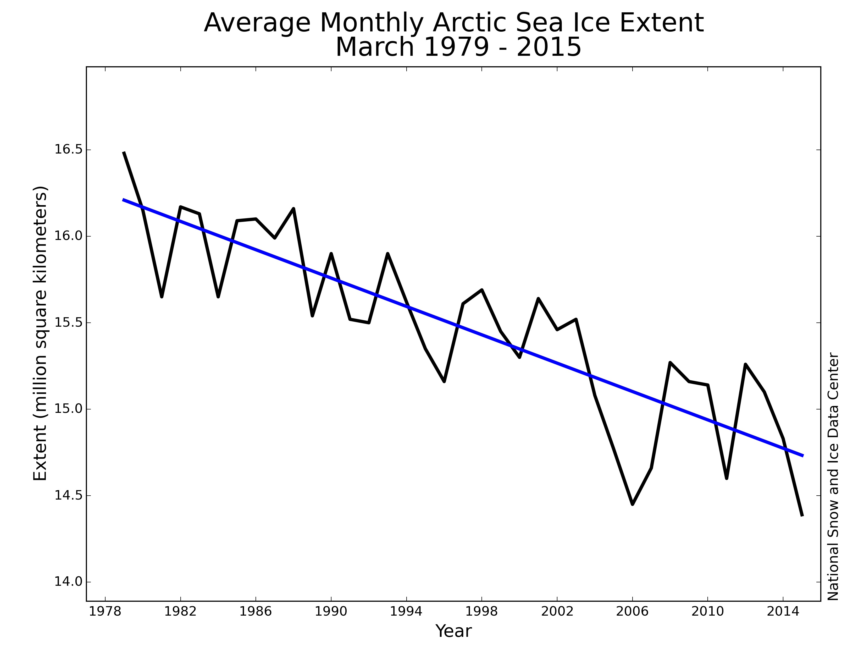
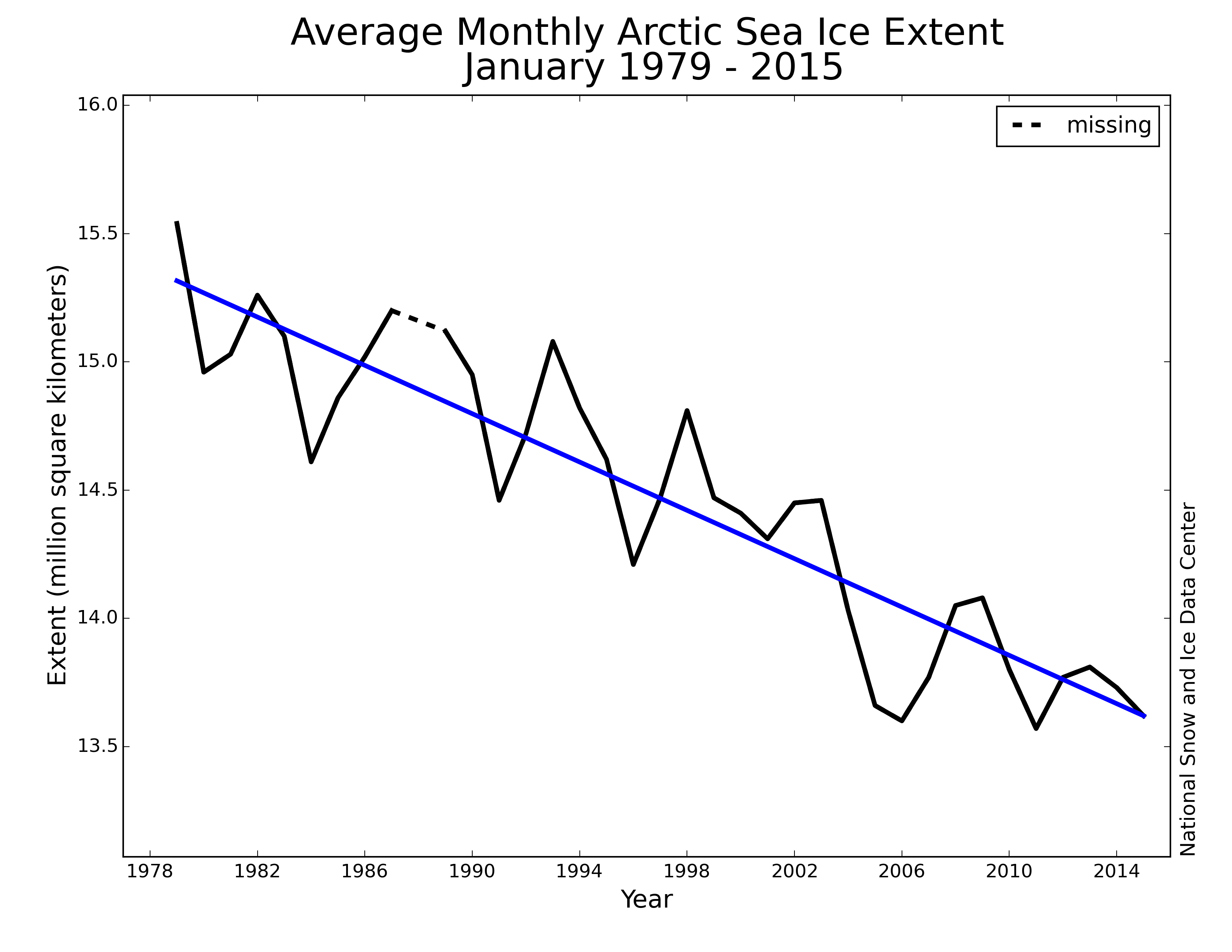
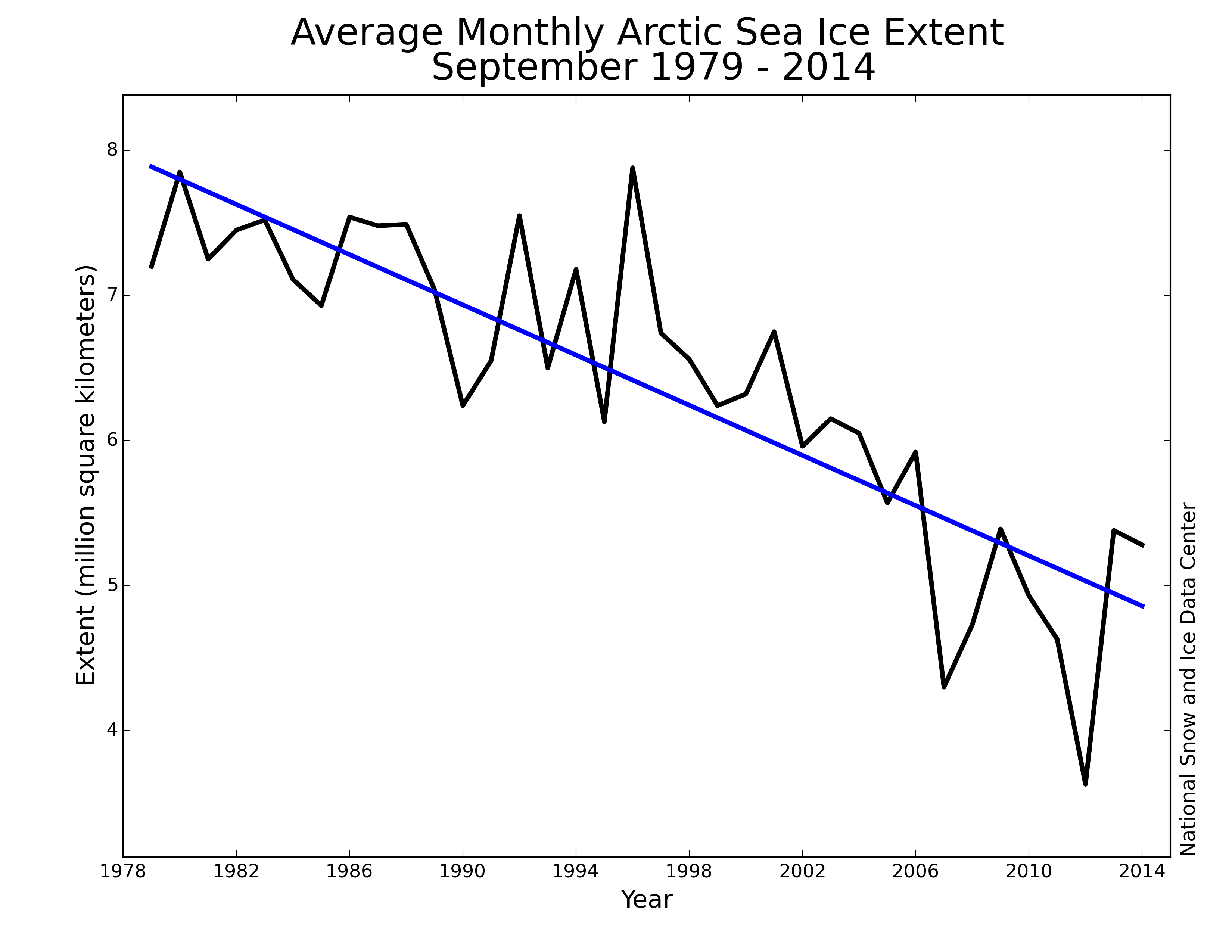
Figure 3. Monthly March ice extent for 1979 to 2015 shows a decline of 2.6% per decade relative to the 1981 to 2010 average.

Credit: National Snow and Ice Data Center
High-resolution image

The monthly average Arctic sea ice extent for March was the lowest in the satellite record. Through 2015, the linear rate of decline for March extent is 2.6% per decade.

Overview of the winter season

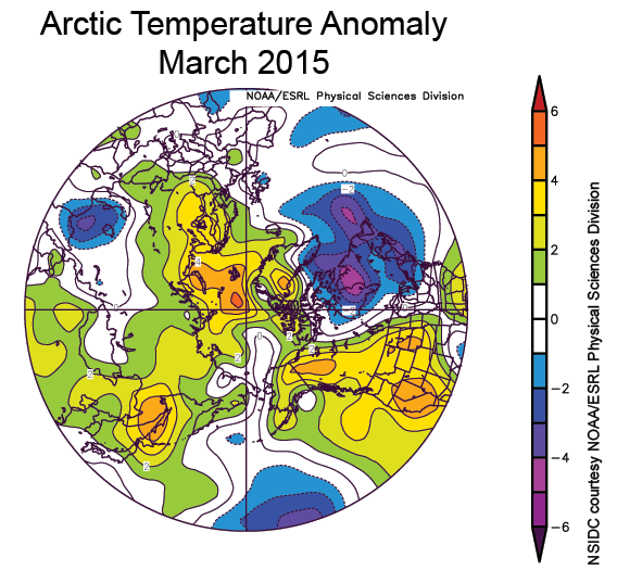
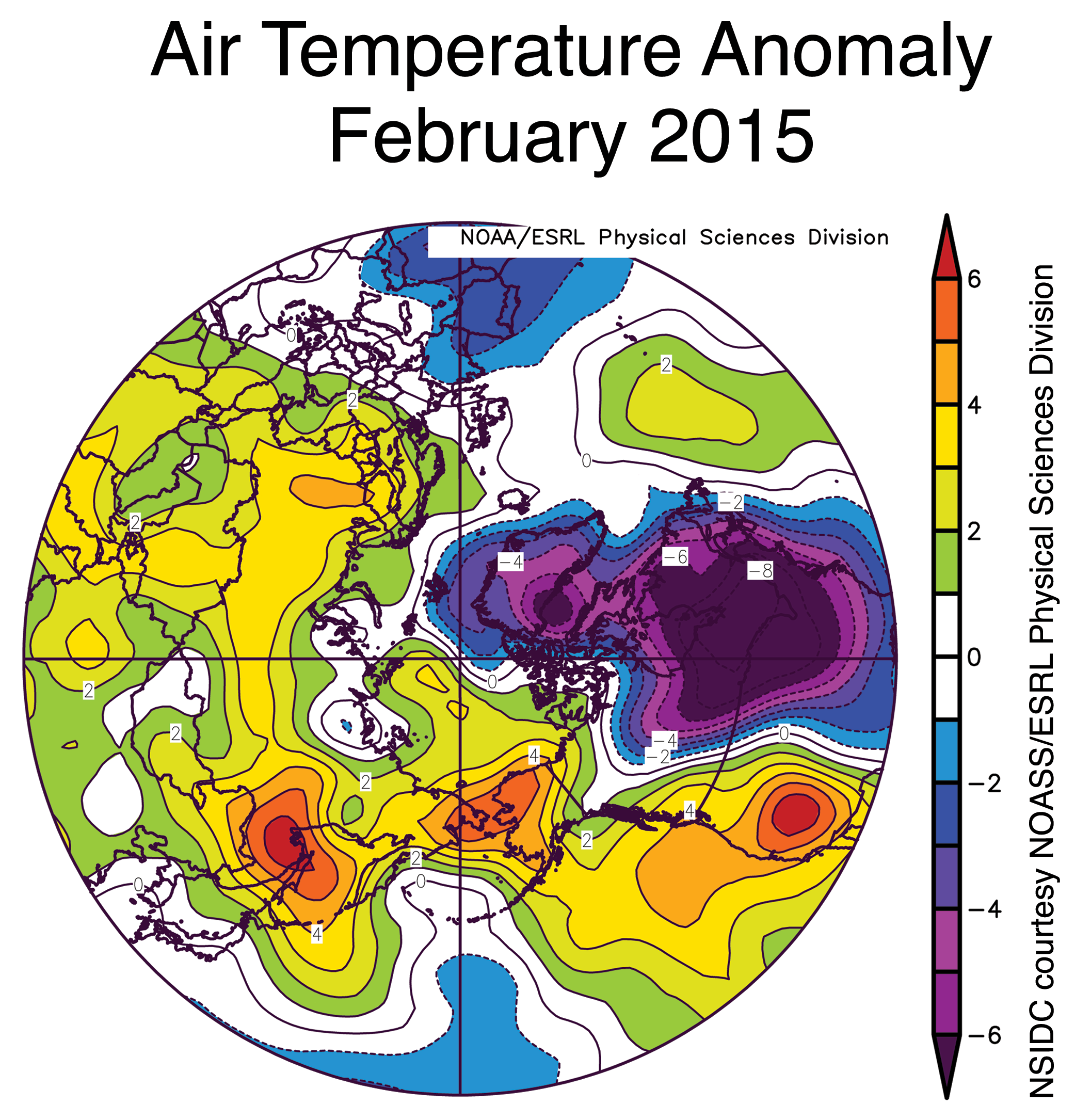
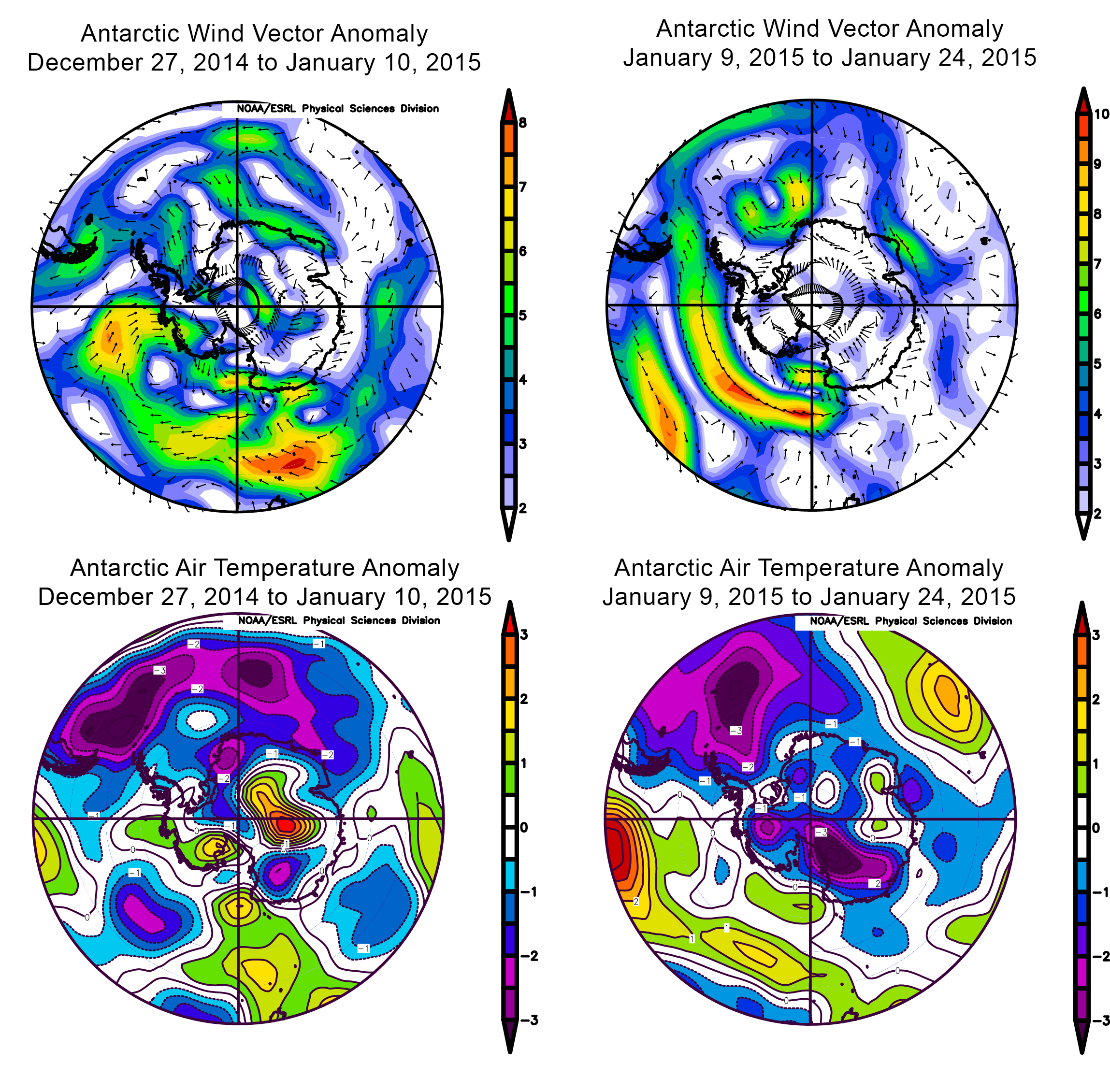
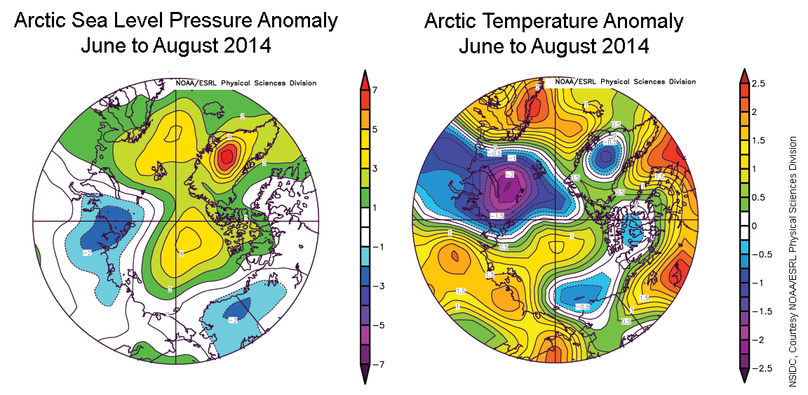
Figure 4. The plot shows Arctic air temperature anomalies at the 925 hPa level in degrees Celsius for March 2015. Yellows and reds indicate higher than average temperatures; blues and purples indicate lower than average temperatures.

Credit: NSIDC courtesy NOAA Earth System Research Laboratory Physical Sciences Division
High-resolution image

As discussed in our previous post, the winter of 2014/2015 was characterized by an unusual pattern of atmospheric circulation, with the jet stream lying well north of its usual location over Eurasia and the North Pacific, and then plunging southwards over eastern North America. This pattern was associated with unusually warm conditions extending across northern Eurasia, the Bering Sea and Sea of Okhotsk, Alaska and into the western part of the United States, contrasting with cold and snowy conditions over the eastern half of the United States. The record low seasonal maximum in ice extent recorded on February 25, 2015 was largely due to low extent in the unusually warm Bering Sea and Sea of Okhotsk. This pattern of atmospheric circulation and temperatures largely continued through March.

Recent work by Dennis Hartmann of the University of Washington suggests that this unusual jet stream pattern was driven, at least in part, by a particular configuration of sea surface temperatures over the tropical Pacific known as the North Pacific Mode, or NPM. The NPM pattern consists of above-average sea surface temperatures in the western Tropical Pacific that extend north and east towards the California coast and across the far northern Pacific Ocean. While the better-known El-Nino-Southern Oscillation (ENSO) pattern has been in a neutral state for the past few winters, the NPM has been in an extreme positive state since the summer of 2013.

The pattern of air temperatures seen this past winter has persisted through March; note the unusually warm conditions over northern Eurasia, Alaska and western North America, contrasting with unusually cold conditions over eastern North America.

Snow cover update

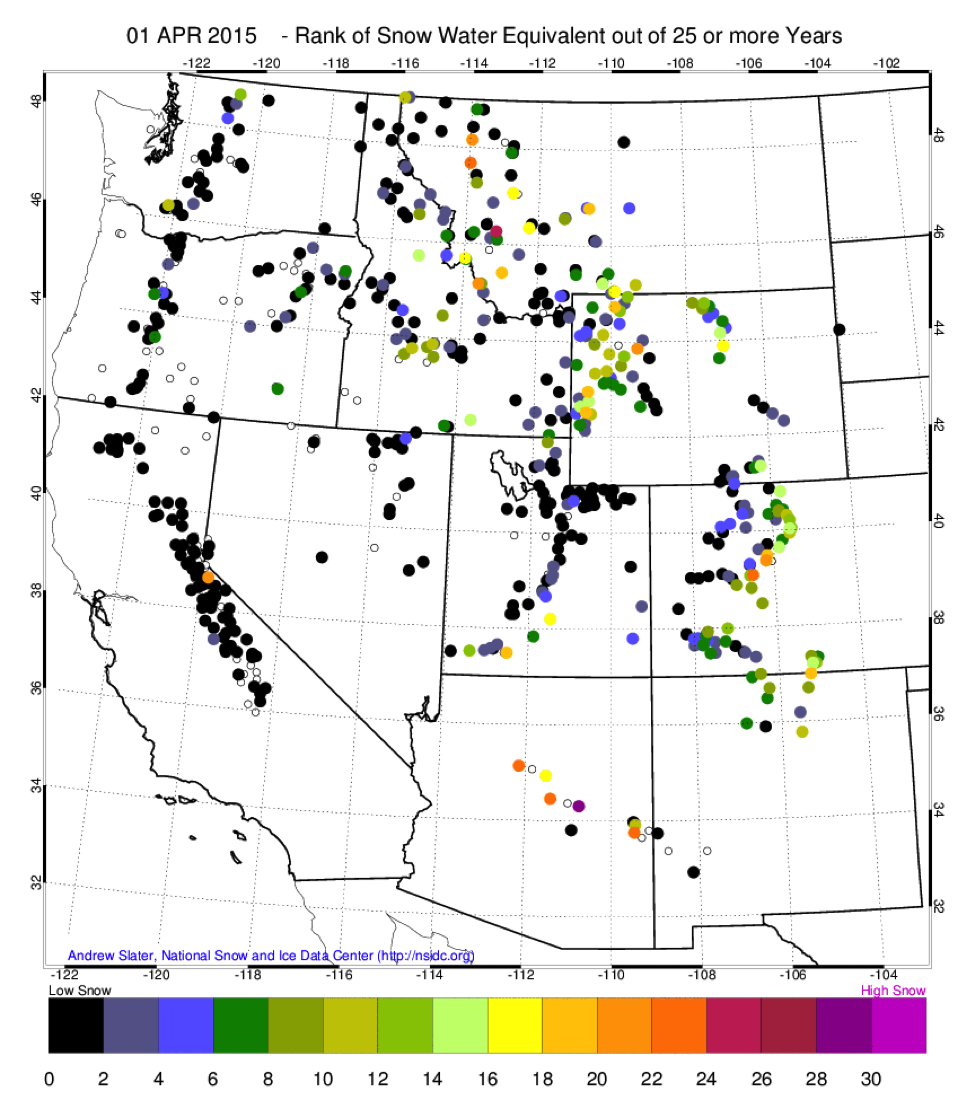
Figure 5. This map shows the rank of snow water equivalent measured at SNOTEL sites across the western U.S. A rank of 1 (black dots) corresponds to the lowest SWE in the SNOTEL record; a rank of 31 (magenta dots) is the highest.

Credit: Andrew Slater, NSIDC
High-resolution image

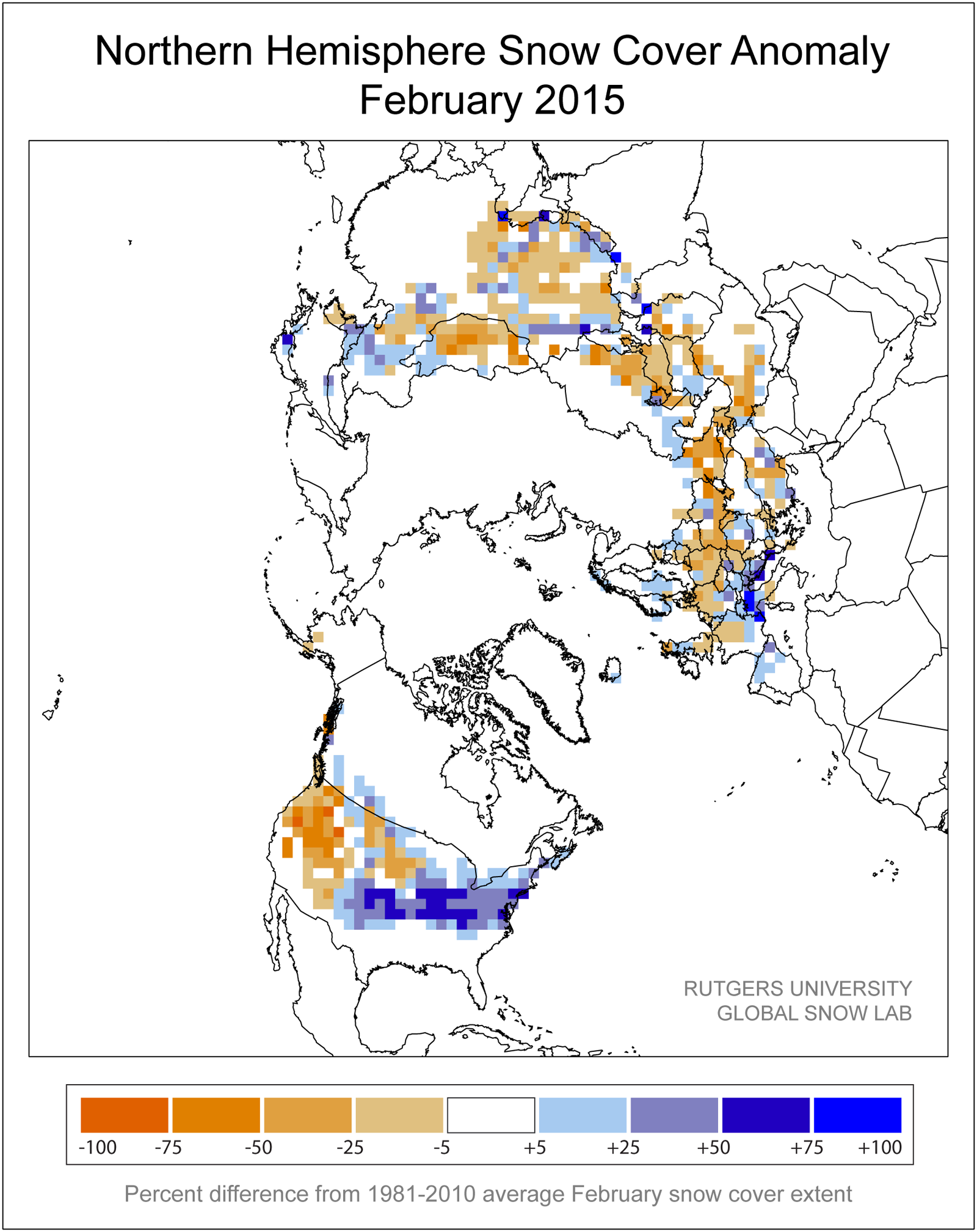
The unusual atmospheric circulation pattern just discussed also helps to explain the snow drought over the western United States. NSIDC scientist Andrew Slater maintains regular updates of western U.S. mountain snowpack conditions using data from the SNOTEL (snowpack telemetry) system – a network of automated sensors that measure snow water equivalent. The automated SNOTEL sites are complemented by snowcourses, where snow water equivalent is measured manually on a periodic basis.

Typically, the snowpack peaks around April 1. As seen in Figure 5, the April 1 snowpack over most of the western United States is far below average. At many sites, snow water equivalent is at historic lows for this time of year. Conditions are somewhat better along the Front Range of Colorado and in Arizona, Wyoming and Montana.

Record warmth in Antarctica

Air temperatures reached record high levels at two Antarctic stations last week, setting a new mark for the warmest conditions ever measured anywhere on the continent. On March 23, at Argentina’s base Marambio, a temperature of 17.4° Celsius (63.3° Fahrenheit) was reached, surpassing a previous record set in 1961 at a nearby base, Esperanza. The old record was 17.1° Celsius (62.8° Fahrenheit). However, Esperanza quickly reclaimed the record a few hours later on March 24, reaching a temperature of 17.5° Celsius (63.5° Fahrenheit).

The cause of these warm conditions is familiar to people living in mountainous regions: a foehn or chinook wind, in which air flows up and over a steep mountain ridge. On the windward side, moisture is wrung out of the air mass in the form of rain or snow. As the air descends on the leeward (downwind) side, it compresses and warms.

This airflow pattern is a key part of the climate conditions that led to past ice shelf disintegrations in the region, such as the dramatic break-up of the Larsen B Ice Shelf in 2002. Air pressure patterns during the event indicated a near-stationary high pressure center in the Drake Passage north of the Antarctic Peninsula, and a strong area of low pressure at the base of the Peninsula, favoring the foehn pattern. Events like this have been recorded by a network of sensors installed by the National Science Foundation LARISSA project.  This network recorded temperatures as high as 16.9° Celsius (62.4° Fahrenheit), westerly winds up to 23 meters per second (45 miles per hour), and a ~100 hour period of temperatures above freezing over the Larsen B area. A recent publication by a colleague at the Scripps Institute of Oceanography describes the impact of foehn or chinook patterns on ice shelf and sea ice stability in the region, making use of the network of Automated Meteorology-Ice-Geophysics Observing Systems (AMIGOS) and other weather sensors in the region.

Further reading

Cape, M., M. Vernet, P. Skvarca, S. Marinsek, T. Scambos, and E. Domack. 2015. Foehn winds link climate-driven warming to coastal cryosphere evolution in Antarctica. Jour. Geophys. Res., Atmospheres, submitted.

Scambos, T., R. Ross, T. Haran, R. Bauer, D.G. Ainley, K.-W. Seo, M. Keyser, A. De, Behar, D.R. MacAyeal. 2013. A camera and multisensor automated station design for polar physical and biological systems monitoring: AMIGOS. Journal of Glaciology, 59 (214), 303-314, doi: 10.3189/2013JoG12J170.

Arctic sea ice extent continues to track well below average, but it is still unclear whether March will see an increase in ice, or establish a record low maximum. Regionally, Arctic ice extent is especially low in the Sea of Okhotsk and the Bering Sea. In the Antarctic, sea ice shrank to the fourth highest minimum in the satellite record.

Overview of conditions

Figure 1. Arctic sea ice extent for February 2015 was 14.41 million square kilometers (5.56 million square miles). The magenta line shows the 1981 to 2010 median extent for that month. The black cross indicates the geographic North Pole. Sea Ice Index data. About the data

Credit: National Snow and Ice Data Center
High-resolution image

Arctic sea ice extent in February averaged 14.41 million square kilometers (5.56 million square miles). This is the third lowest February ice extent in the satellite record. It is 940,000 square kilometers (362,900 square miles) below the 1981 to 2010 long-term average of 15.35 million square kilometers (5.93 million square miles). It is also 50,000 square kilometers (19,300 square miles) above the record low for the month observed in 2005.

With the Arctic Ocean completely ice covered, the remaining areas of potential new ice growth are limited to the margins of the pack in the northern Pacific and northern Atlantic. Sea ice extent is below average across the entire sea ice margin, most prominently along the Pacific sectors. A small region of above-average ice extent is located near Newfoundland and the Canadian Maritime Provinces.

The Arctic maximum is expected to occur in the next two or three weeks. Previous years have seen a surge in Arctic ice extent during March (e.g., in 2012, 2014). However, if the current pattern of below-average extent continues, Arctic sea ice extent may set a new lowest winter maximum.

Conditions in context

Figure 2. The graph above shows Arctic sea ice extent as of March 2, 2015, along with daily ice extent data for four previous years. 2014 to 2015 is shown in blue, 2013 to 2014 in green, 2012 to 2013 in orange, 2011 to 2012 in brown, and 2010 to 2011 in purple. The 1981 to 2010 average is in dark gray. The gray area around the average line shows the two standard deviation range of the data. Sea Ice Index data.

Credit: National Snow and Ice Data Center
High-resolution image

Arctic sea ice extent increased by 429,000 square kilometers (165,600 square miles) during the month of February. This gain was slightly less than the average for the month. While low extent for the Arctic as a whole was largely driven by conditions in the Sea of Okhotsk and the Bering Sea, extent was also slightly below average along the Barents Sea and parts of the East Greenland Sea.

February 2015 compared to previous years

Figure 3. Monthly February ice extent for 1979 to 2015 shows a decline of 2.9% per decade relative to the 1981 to 2010 average.

Credit: National Snow and Ice Data Center
High-resolution image

The monthly average Arctic sea ice extent for February was the third lowest in the satellite record. Through 2015, the linear rate of decline for February extent is 2.9% per decade.

Hot Bering(s)

Figure 4. The plot shows Arctic air temperature anomalies at the 925 hPa level in degrees Celsius for February 2015. Yellows and reds indicate higher than average temperatures; blues and purples indicate lower than average temperatures.

Credit: NSIDC courtesy NOAA Earth System Research Laboratory Physical Sciences Division
High-resolution image

The low ice extent in the Bering Sea and Sea of Okhotsk is linked to unusually warm conditions in the area. February air temperatures at the 925 hPa level were as much as 4 to 6 degrees Celsius (7 to 11 degrees Fahrenheit) above average in the northern Bering Sea, easternmost Siberia, and Sea of Okhotsk.

While these localized hotspots are in part driven by the low sea ice extent and the resulting large heat fluxes from the open water to the atmosphere, they are seen to be part of a broad area of unusually warm conditions extending across most of northern Eurasia, across Alaska, and into the western part of the United States. In contrast, cold and snowy conditions have persisted across the eastern half of North America. Broadly speaking, these opposing patterns of warmth and cold, along with low ice extent in the Sea of Okhotsk and Bering Sea, can be linked to an unusual jet stream pattern, with the jet lying north of its usual location over Eurasia and the North Pacific (meaning that warm air extends further north than is usual), and then plunging southwards over eastern North America.

Snow cover

Figure 5a. This snow cover anomaly map shows the difference between snow cover for February 2015, compared with average snow cover for February from 1981 to 2010. Areas in orange and red indicate lower than usual snow cover, while regions in blue had more snow than normal.

Credit: National Snow and Ice Data Center, courtesy Rutgers University Global Snow Lab
High-resolution image

Figure 5b. This graphs shows snow cover extent anomalies in the Northern Hemisphere for February from 1967 to 2015. The anomaly is relative to the 1981 to 2010 average.

Credit: National Snow and Ice Data Center, courtesy Rutgers University Global Snow Lab
High-resolution image

This unusual jet stream pattern is clearly manifested in the pattern of Northern hemisphere snow cover for February. Snow extent was well above average over the northeastern U.S. However, the western U.S. and Northern Rockies saw less snow cover than average, especially along the Pacific coast where it has been particularly warm and severely dry. While the Tibetan Plateau saw a somewhat more extensive snow cover than average in December and January, extent for Tibet and Eurasia as a whole was below average in February. Higher-than-average snow cover in the eastern U.S. expanded and became more pronounced this month as well. All of these are continuations of the basic pattern seen in December and January, although the pattern of extensive snow over the northeastern U.S. became more pronounced this month. The low snow cover extent in much of Eurasia is consistent with the warmer-than-average conditions there as described above.

Seasonal Antarctic minimum reached

Figure 6a. This figure shows the concentration anomaly for February 2015 monthly average extent relative to the 1981 to 2010 average. Sea Ice Index data. About the data

Credit: National Snow and Ice Data Center
High-resolution image

Figure 6b. Monthly Antarctic February ice extent for 1979 to 2015 shows a trend of 5.0% per decade relative to the 1981 to 2010 average.

Credit: National Snow and Ice Data Center
High-resolution image

Antarctic sea ice extent reached its annual minimum, dipping to 3.58 million square kilometers (1.38 million square miles) on February 20. This is the fourth highest summer minimum extent on record, trailing behind 2008 (3.75 million square kilometers or 1.44 million square miles, highest), 2013, and 2003. The 2014 Antarctic minimum ranked the fifth highest (3.54 million square kilometers or 1.36 million square miles). For the month as a whole, February 2015 has the sixth highest ice extent (3.8 million square kilometers or 1.46 million square miles). The sea ice extent trend for February for 1979 to 2015 shows an increase of 5.0%  per decade. However, Antarctica’s sea ice extent is highly variable. As recently as 2011, Antarctic sea ice extent was at near-record low levels for the summer minimum.

Nevertheless, the recent series of high-ice-extent minima is part of a remarkable recent uptick in extent year-round for Antarctica, dominated by extensive ice in both the Weddell Sea (south of Africa) and the Ross Sea (south of New Zealand). Sea ice in the eastern Weddell Sea presently extends several hundred kilometers further north and east of its typical extent, while ice extent in the Ross Sea is presently near average. The debate continues regarding the cause of the recent Antarctic trends, but the best explanation so far involves a combination of strengthening low pressure in the eastern Ross Sea (the Amundsen Sea Low) and the eastern Weddell Sea, and a persistently positive phase of the Southern Annular Mode. The freshening of surface seawater around Antarctica may also play a role.

Global sea ice trends

Claire Parkinson of NASA recently presented the global average (Arctic plus Antarctic) trend in sea ice extent for the period 1979 to 2013. Overall, global sea ice has declined, despite the positive trend in Antarctic extent. The annual average trend is -35,000 square kilometers (-13,500 square miles) per year, or about -1.5% per decade. The strong Arctic decline in September leads to the largest magnitude monthly trend for global sea ice in that month, at -68,000 square kilometers (-26,300 square miles) per year, or -2.6% per decade. See the NSIDC FAQ on global sea ice here.

Further reading

Parkinson, C. L. 2014. Global sea ice coverage from satellite data: annual cycle and 35-year trends. Journal of Climate, doi: 10.1175/JCLI-D-14-00605.1.

Arctic sea ice extent was the third lowest for the month of January. Ice extent remained lower than average in the Bering Sea and Sea of Okhotsk, while ice in the Barents Sea was near average. Antarctic sea ice extent declined rapidly in late January, but remains high.

Overview of conditions

Figure 1. Arctic sea ice extent for January 2015 was 13.62 million square kilometers (5.26 million square miles). The magenta line shows the 1981 to 2010 median extent for that month. The black cross indicates the geographic North Pole. Sea Ice Index data. About the data

Credit: National Snow and Ice Data Center
High-resolution image

Sea ice extent in January averaged 13.62 million square kilometers (5.26 million square miles). This is 910,000 square kilometers (351,000 square miles) below the 1981 to 2010 long-term average of 14.53 million square kilometers (5.61 million square miles), and 50,000 square kilometers (19,000 square miles) above the record low for the month observed in 2011.

This below-average Arctic extent is mainly a result of lower-than-average extent in the Bering Sea and the Sea of Okhotsk. On the Atlantic side, Barents Sea ice extent is near average. This is in sharp contrast to the general pattern seen since 2004 of below average extent in this region, but above average extent in the Bering Sea. Ice extent is also near average in the East Greenland Sea, Baffin Bay and the Labrador Sea.

Conditions in context

Figure 2. The graph above shows Arctic sea ice extent as of February 2, 2015, along with daily ice extent data for four previous years. 2014 to 2015 is shown in blue, 2013 to 2014 in green, 2012 to 2013 in orange, 2011 to 2012 in brown, and 2010 to 2011 in purple. The 1981 to 2010 average is in dark gray. The gray area around the average line shows the two standard deviation range of the data. Sea Ice Index data.

Credit: National Snow and Ice Data Center
High-resolution image

During most of January, the Arctic Oscillation (AO) was in a strongly positive phase. When the AO is in a positive phase, sea level pressure in the Arctic is particularly low, and sea level pressure is relatively high in the middle latitudes of the Northern Hemisphere. Variability in Arctic sea ice conditions is strongly influenced by the phase of the AO. Typically, during the positive phase of the AO, surface winds push ice away from the shores of Siberia, leading to the formation of more young, thin ice that is prone to melting out in summer. The positive phase also tends to increase the transport of thick, multiyear ice out of the Arctic through Fram Strait.

Air temperatures (at the 925 millibar level, about 3,000 feet above the surface) were mostly above average over most of the Arctic Ocean, with positive anomalies of 4 to 6 degrees Celsius (7 to 11 degrees Fahrenheit) over the Chukchi and Bering seas on the Pacific side of the Arctic, and also over the East Greenland Sea on the Atlantic side.

January 2015 compared to previous years

Figure 3. Monthly January ice extent for 1979 to 2015 shows a decline of 3.2% per decade relative to the 1981 to 2010 average.

Credit: National Snow and Ice Data Center
High-resolution image

Arctic sea ice extent for January was the third lowest in the satellite record. Through 2015, the linear rate of decline for January extent over the satellite record is 3.2% per decade.

Barents Sea ice variability

Figure 4. The graph shows Barents Sea ice area (blue line) and ocean temperatures in the Barents Sea Opening (red line) from 1980 to 2015. The sea ice area tends to be smaller for higher Atlantic water temperatures, with a lag of 1 to 2 years (note the reversed scale for Atlantic water temperatures). The data are based on Årthun et al. (2012), who find that the ocean temperature largely reflects changes in volume of Atlantic water inflow. Sea ice area anomalies are from the NASA Team algorithm (Cavalieri et al., 1996), provided by the National Snow and Ice Data Center. Ocean temperature has been sampled by the Institute of Marine Research (IMR), Norway, and is a section between Norway and Bear Island (BSO; 71.5-73.5N, 20E).

Credit: Ingrid Onarheim, Bjerknes Centre for Climate Research
High-resolution image

Variability in winter sea ice in the Barents Sea largely reflects ocean heat transport. The inflow of Atlantic water between Norway and Bear Island (the Barents Sea Opening or BSO) is the Barents Sea’s main oceanic heat source. Because there are no significant freshwater sources reaching the central Barents Sea, this warm Atlantic water extends to the surface and readily impacts the sea ice. This contrasts with the rest of the Arctic Ocean, where the Atlantic water lies well beneath the slightly fresher polar surface layer. The import of sea ice in the northern straits is also small, around 20% of the sea ice area exported southwards in the Fram Strait, meaning that the Barents Sea primarily consists of thin, first-year ice. Thus, periods with large volumes of warm Atlantic water entering into the Barents Sea are correlated with less sea ice formation and overall less sea ice extent.

Variations in winter ice extent in the Barents Sea are well correlated with variations in overall Arctic sea ice extent, as assessed over the satellite record. This winter is an exception. Sea ice extent in the Barents Sea is fairly high compared to recent years, while it is low for the Arctic as a whole. According to colleagues at the University of Bergen, this is due to a reduced overall inflow of Atlantic waters. A maximum in the ocean heat transport occurred in the mid 2000s, yet since then, the inflow has in general lessened, both along the Norwegian coast, through the Fram Strait, and through the Barents Sea Opening between Norway and Bear Island. Variations in Atlantic inflow is a focus of ongoing research at the Bjerknes Centre in Bergen, as well as in other research centers in Europe.

Antarctic sea ice declines rapidly, still high

Figure 5a. The graph above shows Antarctic sea ice extent as of February 2, 2015, along with daily ice extent data for four previous years. 2014 to 2015 is shown in blue, 2013 to 2014 in green, 2012 to 2013 in orange, 2011 to 2012 in brown, and 2010 to 2011 in purple. The 1981 to 2010 average is in dark gray. The gray area around the average line shows the two standard deviation range of the data. Sea Ice Index data.

Credit: National Snow and Ice Data Center
High-resolution image

Antarctic sea ice extent reached record high levels for late December 2014 and early January 2015, peaking around January 10 at more than 2.5 million square kilometers (965,000 square miles) above the 1981 to 2010 average, and 1.05 million square kilometers (580,000 square miles) above the previous record (2014) for that date. As noted last month, the largest excursions are occurring in the northern Weddell Sea and the northern Ross Sea. After January 10, and particularly after January 19, sea ice extent dropped rapidly (~250,000 square kilometers, or 96,500 square miles, per day), and large areas of the northern Ross Sea became ice free. The northern Weddell region still has a very large ice extent relative to average conditions.

Figure 5b. These images show Antarctic wind vector (top) and air temperature (bottom) anomalies for late December 2014 to early January 2015, compared to 1981 to 2010 averages.

Credit: NOAA ESRL Physical Sciences Division
High-resolution image

Weather conditions during late December and January help to explain these changes. In the northern Weddell Sea, southerly winds (more so than average) and cool conditions relative to the 1981 to 2010 average prevailed for late December and all of January, and sea ice there remained high relative to long-term averages for the month. For the northern Ross Sea, air temperatures at the 925 hPa level have been slightly above average for the entire period, but winds in this area shifted during January, from southerly (pushing ice outward) to northwesterly. The combination of northerly winds and slightly warm conditions seems to have reduced the ice extent anomaly significantly in this sector.

Further reading

Smedsrud, L.H., I. Esau, R. B. Ingvaldsen, T. Eldevik, P. M. Haugan, C. Li, V. S. Lien, A. Olsen, A. M. Omar, O. H. Otterå, B. Risebrobakken, A. B. Sandø, V. A. Semenov, and S. A. Sorokina. 2013. The role of the Barents Sea in the Arctic climate system.
Reviews of Geophysics, 51, doi:10.1002/rog.20017.

Årthun, M., T. Eldevik, L. H. Smedsrud, Ø. Skagseth, and R. B. Ingvaldsen. 2012.
Quantifying the Influence of Atlantic Heat on Barents Sea Ice Variability and Retreat. Journal of Climate, Volume 25, pp. 4736-4743, doi:10.1175/JCLI-D-11-00466.1.

Schauer, U. and A. Beszczynska-Möller. 2009. Problems with estimation and interpretation of oceanic heat transport – conceptual remarks for the case of Fram Strait in the Arctic Ocean, Ocean Sci., 5, 487–494.

Arctic sea ice extent remained about a standard deviation below average for the month of December. Compared to recent years, 2014 as a whole was rather unremarkable. The bigger story was the record high extents observed in the Antarctic through more than half of the year. At year’s end, Antarctic sea ice extent was again at a record high, but poised for a rapid decline as the austral summer wears on.

Overview of conditions

Figure 1. Arctic sea ice extent for December 2014 was 12.52 million square kilometers (4.83 million square miles). The magenta line shows the 1981 to 2010 median extent for that month. The black cross indicates the geographic North Pole. Sea Ice Index data. About the data

Credit: National Snow and Ice Data Center
High-resolution image

Sea ice extent in December averaged 12.52 million square kilometers (4.83 million square miles). This is 540,000 square kilometers (208,495 square miles) below the 1981 to 2010 long-term average of 13.06 million square kilometers (5.04 million square miles) and 500,000 square kilometers (193,051 square miles) above the record low for the month observed in 2010.

Both Hudson Bay and Baffin Bay are now essentially completely ice covered. On the Atlantic side, recent winters have been characterized by reduced winter ice extent in the Kara and Barents seas. This is not the case for the winter of 2014 to 2015.

The only two regions where extent is notably below average are in the Bering Sea and the Sea of Okhotsk. This contrasts with recent winters when ice extent has been greater than average in the Bering Sea.

Conditions in context

Figure 2. The graph above shows Arctic sea ice extent as of January 4, 2015, along with daily ice extent data for four previous years. 2014 to 2015 is shown in blue, 2013 to 2014 in green, 2012 to 2013 in orange, 2011 to 2012 in brown, and 2010 to 2011 in purple. The 1981 to 2010 average is in dark gray. The gray area around the average line shows the two standard deviation range of the data.Sea Ice Index data.

Credit: National Snow and Ice Data Center
High-resolution image

Sea ice extent grew 2.00 million square kilometers (772,000 square miles) during the month of December. This was about average for the month. Throughout the month, daily extents were about one standard deviation below 1981 to 2010 averages. This occurred despite the fairly warm conditions over the Eurasian side of the Arctic Ocean. As averaged over the month, air temperatures at the 925 hPa level in the Laptev and East Siberian seas were up to 5 degrees Celsius (9 degrees Fahrenheit) above average, linked to a region of unusually high pressure in the region that led to southerly winds.

December 2014 compared to previous years

Figure 3. Monthly December ice extent for 1979 to 2014 shows a decline of 3.4% per decade relative to the 1981 to 2010 average. The dashed line indicates a period of missing data from December 2, 1987 through January 12, 1988.

Credit: National Snow and Ice Data Center
High-resolution image

Arctic sea ice extent for December was the ninth lowest in the satellite record. Through 2014, the linear rate of decline for December extent over the satellite record is 3.4% per decade.

2014 in review

Compared to recent years, sea ice conditions observed throughout 2014 were largely unremarkable. Throughout the year, extent for the Arctic as a whole remained below average, but generally within two standard deviations of the average. The maximum extent observed on March 21 of 14.91 million square kilometers (5.76 million square miles) was the fifth lowest in the satellite record, with the minimum extent observed on September 17 of 5.02 million square kilometers (1.94 million square miles) being the sixth lowest on record. One event of note was in the Laptev Sea, where during August, open water was observed to extend to about 85 degrees latitude, less than 560 kilometers (350 miles) from the North Pole.

Summer weather conditions, which are known to strongly influence September minimum ice extent, were also largely unremarkable in 2014. Compared to the long term (1981 to 2010) climatology, sea level pressure over the period June through August 2014 was higher than average over much of the central Arctic Ocean, the Atlantic sector of the Arctic, and Greenland. While air temperatures at the 925 hPa level (approximately 3,000 feet altitude) were slightly above average over part of the central Arctic Ocean, they were below average over the Kara Sea and just north of Alaska.

By sharp contrast, sea ice in Antarctica was at satellite-era record high daily levels for much of 2014. On September 22, 2014, Antarctic ice extent reached 20.11 million square kilometers (7.76 million square miles). This was the first year in the modern satellite record that Antarctic ice extent climbed above 20 million square kilometers (7.72 million square miles).

As the year drew to a close, sea ice extent again reached record high levels for the date by declining far more slowly than usual. Extent anomalies are particularly large in the Ross Sea and Amundsen Sea regions, and in the northern Weddell Sea—areas that have been anomalously high for most of the calendar year. However, sea ice concentration in both these regions is now quite low, that is, the sea ice pack is loose and open. This is characteristic of dispersal of the ice by storms, and indeed strong low pressure anomalies were present in the eastern Ross Sea and northern Weddell Sea in the second half of December. The extent of this loose sea ice pack far to the north makes it likely that a rapid decline will occur as warmer summer weather arrives.

Losing the memory of low extent

Figure 4. This graph shows future projections of September sea ice extent under various future greenhouse gas emission levels. Limiting the warming in 2100 to about 1 to 2 degrees Celsius (2 to 4 degrees Fahrenheit) under the RCP2.6 emission scenario would help to stabilize ice conditions at levels seen today. The RCP8.5 emission scenario (warming by about 4 degrees Celsius 0r 7 degrees Fahrenheit by the end of this century) would result in a seasonally ice-free Arctic by the end of this century.

Credit: Julienne Stroeve
High-resolution image

In September of 2014, the Royal Society of London held a workshop focused on the reduction in Arctic sea ice extent. One outcome of this meeting was a greater understanding of the overall trajectory of September ice extent. In a nutshell, it appears that very large departures from the overall downward trend in September extent are unlikely to persist into the following September. If a given September has very low ice extent, strong winter heat loss results in strong ice growth, so that the “memory” of the low ice September ice extent is lost. If a given September has a high ice extent, winter heat loss is more limited, meaning less ice growth. Consequently, while there can be large departures from year to year from the downward linear trend in ice extent (e.g., September 2012 compared to 2014), the natural tendency is for the large departure to dampen out, so that, overall, ice extent stays on the long-term downward trajectory that will eventually lead to seasonally ice free conditions as the Arctic continues to warm in response to rising atmospheric concentrations of Greenhouse gases.

While the U.S. experienced extreme weather in November, conditions in the Arctic were fairly ordinary. Arctic sea ice in November followed a fairly average growth pace. Ice extent was near average over much of the Arctic with only the Chukchi Sea and Davis Strait showing below average ice conditions.

Overview of conditions

Figure 1. Arctic sea ice extent for November 2014 was 10.36 million square kilometers (4.00 million square miles). The magenta line shows the 1981 to 2010 median extent for that month. The black cross indicates the geographic North Pole. Sea Ice Index data. About the data

Credit: National Snow and Ice Data Center
High-resolution image

Sea ice extent in November averaged 10.36 million square kilometers (4.00 million square miles). This is 630,000 square kilometers (243,000 square miles) below the 1981 to 2010 long-term average of 10.99 million square kilometers (4.24 million square miles) and 520,000 square kilometers (201,000 square miles) above the record low for the month observed in 2006.

Arctic sea ice extent continued to increase throughout the month of November. By the end of the month, most of the Arctic Ocean was covered by ice, the exception being the Chukchi Sea that remained unusually ice free for this time of year. Ice also began to extend into Hudson Bay and Baffin Bay, although ice growth was slower than average in Davis Strait. The near-average ice conditions in the East Greenland, Barents and Kara seas have not been seen in the last few winters, and is the reason that overall extent for November is higher than in recent years.

Conditions in context

Figure 2. The graph above shows Arctic sea ice extent as of November 30, 2014, along with daily ice extent data for four previous years. 2014 is shown in blue, 2013 in green, 2012 in orange, 2011 in brown, and 2010 in purple. The 1981 to 2010 average is in dark gray. The gray area around the average line shows the two standard deviation range of the data. Sea Ice Index data.

Credit: National Snow and Ice Data Center
High-resolution image

Sea ice extent grew 2.15 million square kilometers (830,000 square miles) during the month of November. This was about average for the month and substantially slower than observed in 2012. While the month started with 1.17 million square kilometers (452,000 square miles) more ice in 2014 than on November 1, 2012, by the end of the month, the difference between 2014 and 2012 had closed to only 416,000 square kilometers (161,000 square miles). The difference in November ice growth between 2012 and 2014 reflects the larger area of open water at the end of summer 2012. With more open water, there was a larger area for new ice to grow.

November 2014 compared to previous years

Figure 3. Monthly November ice extent for 1979 to 2014 shows a decline of 4.7% per decade relative to the 1981 to 2010 average.

Credit: National Snow and Ice Data Center
High-resolution image

Arctic sea ice extent for November was the 9th lowest in the satellite record. Through 2014, the linear rate of decline for November extent over the satellite record is 4.7% per decade.

Arctic amplification and mid-latitude weather extremes

Figure 4. This plot of average surface air temperatures from November 17 to 19, 2014 over North America during a polar outbreak shows unusually cold air reaching down into the U.S. Temperatures are in degrees Kelvin. Blues and purples indicate sub-freezing temperatures.

Credit: NSIDC/NOAA ESRL Physical Sciences Divisionr
High-resolution image

Last month we discussed how the extra heat stored in ice-free areas of the ocean during recent summers is released back to the atmosphere as the ice begins to re-form, leading to amplified warming in the Arctic atmosphere. The impact of this warming and its potential impacts on mid-latitude weather patterns and extreme weather events is an active area of research.

This November has been particularly notable for severe weather in the U.S., with a very strong storm in the Bering Sea affecting the Aleutian Islands of western Alaska* (a remnant of Typhoon Nuri that tracked from the tropics through the Aleutians), record-setting low temperatures in the upper plains, and epic lake-effect snow near Buffalo, N.Y. Such individual events cannot be directly linked to climate change, let alone specifically to sea ice loss.

*Correction, December 16, 2014: Adjusted the wording here to make clear that the storm did not affect mainland Alaska, but only the Aleutians.

New research this year from Japanese scientists (Mori et al., 2014) provides support for the hypothesis, put forward by Jennifer Francis of Rutgers University and Steve Vavrus of the University of Wisconsin, that the warming Arctic is contributing to an increasing waviness of the jet stream with the potential for more extreme weather events, including cold outbreaks in the lower 48 U.S. and Eurasia that have been seen in recent years. However, while there is some evidence of this connection, it is not conclusive and many scientists remain skeptical of a link between Arctic sea ice and mid-latitude weather.

Antarctica watch

Figure 5. Antarctic sea ice extent for November 2014 was 16.63 million square kilometers (6.42 million square miles). The magenta line shows the 1981 to 2010 median extent for that month. The black cross indicates the geographic South Pole. Sea Ice Index data. About the data

Credit: National Snow and Ice Data Center
High-resolution image

Antarctic sea ice has continued to decline at a faster-than-average pace (approximately 122,000 square kilometers, or 47,100 square miles per day through the month of October, compared to the average rate of 112,000 square kilometers or 43,200 square miles per day), and is now about 650,000 square kilometers (251,000 square miles) below the level for the date recorded in 2013. Currently ice extent remains about 700,000 square kilometers (270,000 square miles) higher than the 1981 to 2010 average for this time of year. Large reductions in the Bellingshausen Sea and the southern Indian Ocean were the main causes of the Antarctic-wide decrease, driven in large part by persistent northerly winds. Air temperatures over the Southern Ocean for the month were near average in nearly all areas. On the icy continent itself, cool conditions prevailed over the Antarctic Peninsula and West Antarctica (1 to 2 degrees Celsius, or 1.8 to 3.6 degrees Fahrenheit below average) while warm conditions were the rule in the Eastern Hemisphere section (2 to 4 degrees Celsius, or 3.6 to 7.2 degrees Fahrenheit above average).

Reference

Mori, M., M. Watanabe, H. Shiogama, J. Inoue, and M. Kimoto, 2014. Robust Arctic sea-ice influence on the frequent Eurasian cold winters in past decades. Nature Geoscience, vol. 7, pp. 869-873.

Arctic sea ice continued to expand throughout the month of October, remaining at near-average levels on the Atlantic side and below average on the Pacific side. In the Southern Hemisphere, Antarctic sea ice has declined after reaching its record maximum in October and is now nearly within two standard deviations of the long-term average.

Overview of conditions

Figure 1. Arctic sea ice extent for October 2014 was 8.06 million square kilometers (3.11 million square miles). The magenta line shows the 1981 to 2010 median extent for that month. The black cross indicates the geographic North Pole. Sea Ice Index data. About the data

Credit: National Snow and Ice Data Center
High-resolution image

Sea ice extent in October averaged 8.06 million square kilometers (3.11 million square miles). This is 850,000 square kilometers (328,000 square miles) below the 1981 to 2010 long-term average of 8.91 million square kilometers (3.44 million square miles) and 1.29 million square kilometers (498,000 square miles) above the record low for the month observed in 2007.

Arctic sea ice extent continued to increase throughout the month of October. Ice extent in the Pacific side remains below average. Areas in the Beaufort Sea along the Canadian and Alaskan coasts, and in the Chukchi Sea along the coast of Siberia were still ice free at the end of October. The image of monthly average sea ice extent (Figure 1) shows a large polynya within the East Siberian Sea, but this area is now covered by ice. On the Atlantic side, extent remains at near-average levels.

Conditions in context

Figure 2. The graph above shows Arctic sea ice extent as of November 3, 2014, along with daily ice extent data for four previous years. 2014 is shown in blue, 2013 in green, 2012 in orange, 2011 in brown, and 2010 in purple. The 1981 to 2010 average is in dark gray. The gray area around the average line shows the two standard deviation range of the data. Sea Ice Index data.

Credit: National Snow and Ice Data Center
High-resolution image

Through the month of October, the Arctic gained 3.39 million square kilometers (1.31 million square miles) of ice. This is faster than the average rate of ice gain for the month of October, but slower than the rate of ice gain seen in October 2012, after the record minimum of September 2012, and other recent Octobers.

Temperatures at the 925 hPa level show that the Arctic was 1 to 4 degrees Celsius (2 to 7 degrees Fahrenheit) higher than average everywhere, except in the Kara and Barents seas where air temperatures were 1 to 3 degrees Celsius (2 to 5 degrees Fahrenheit) lower than average. Lower than average temperatures in this region were also a persistent feature of summer 2014 and helped maintain a more extensive ice cover in the region than in recent summers.

Warm conditions were partly a result of the ocean releasing the heat gained during summer back to the atmosphere. In addition, sea level pressures were higher than average over the central Arctic Ocean and the Barents Sea, reflecting the negative phase of the Arctic Oscillation .

October 2014 compared to previous years

Figure 3. Monthly October ice extent for 1979 to 2014 shows a decline of 6.9% per decade relative to the 1981 to 2010 average.

Credit: National Snow and Ice Data Center
High-resolution image

Due to the relatively rapid ice growth during October, Arctic sea ice extent for October 2014 was the 6th lowest in the satellite record. Through 2014, the linear rate of decline for October Arctic ice extent over the satellite record is 6.9% per decade.

Amplified autumn warming

Figure 4. This figure shows average air temperature anomalies for October 2014 at each latitude from 50 North (left side of axis) to 90 North (right side of axis). The Y axis shows air pressure in millibars, indicating height above the surface.

Credit: NSIDC courtesy NOAA Earth System Research Laboratory Physical Sciences Division
High-resolution image

Projections of climate change through the rest of the century show amplified warming in the Arctic compared to the rest of the planet. While there are a number of reasons for this, sea ice loss plays a strong role. With less ice in spring and summer, the upper ocean (the top 20 meters, or 66 feet) gains more heat through absorption of solar radiation. For the ocean surface to refreeze in autumn and winter, the ocean must first lose this extra heat. This is manifested as strong surface warming over the areas of sea ice loss during autumn. While the warming is greatest near the surface, the warming can extend to a considerable height in the atmosphere.

This October shows the expected pattern of amplified warmth. Warming was greatest near the surface at high latitudes (5 degrees Celsius, or 9 degrees Fahrenheit above average) and extended upwards to the 700 hPa level, roughly 3,000 meters (9,842 feet) above the surface. This pattern is similar to that observed in October 2007 and 2009. However, in other recent years the location of the warmest surface conditions shifted further south, or did not extend as far up in the atmosphere. Such variations point to the influence of other factors, including patterns of atmospheric circulation, cloud cover, and atmospheric humidity.

Arctic sea ice and the Madden-Julian Oscillation

Variations in large-scale atmospheric circulation patterns, such as the Arctic Oscillation , are known to affect the sea ice cover. These variations alter wind patterns that affect ice motion and bring in warm or cold air that influence ice melt and growth. For example, during a positive Arctic Oscillation phase, changes in the wind field help to push ice away from the coast of Siberia, allowing new ice to form and increasing the transport of ice out of Fram Strait. In the winters of the late 1980s and early 1990s, the Arctic Oscillation was in a persistent positive phase, helping to transport a large amount of thick, multiyear ice out of the Arctic through Fram Strait and leaving behind thinner ice that more easily melted the following summers.

A new study looks at the impact of a different mode of large-scale atmospheric variability, the Madden-Julian Oscillation, which appears to impact the ice cover on a shorter 30- to 90-day time scale. The Madden-Julian Oscillation is primarily driven by convection in the tropics, but causes changes in atmospheric circulation that impact the high latitudes. The impact on sea ice was found to be stronger during the winter season than in summer. It affected both the Atlantic and Pacific sectors and was confined to the marginal ice zone. The impact on sea ice also varies regionally, often showing opposing effects, such as between the Barents and Greenland seas in winter.

Large Antarctic sea ice variability

Figure 5. This image compares Antarctic sea ice extent for September 2014 (blue line) with extent for September 1964 (red line) and August 1966 (black line). The dotted ellipse marked A shows the eastern Weddell Sea and the dotted ellipse marked B shows the eastern Ross Sea.

Credit: National Snow and Ice Data Center
High-resolution image

After reaching a new record maximum extent this September, Antarctic sea ice extent has quickly declined, and is now back to levels seen in 2013 at this time of year. While almost the entire perimeter of Antarctica’s sea ice retreated slightly, two regions showed a larger retreat after the maximum: the eastern Weddell Sea (dotted ellipse marked A in Figure 5) and the eastern Ross Sea (dotted ellipse marked B in Figure 5). Both were areas of unusually extensive sea ice cover, and they contributed significantly to the record-setting level of ice extent in September. Weather patterns thirty days after the maximum changed markedly, with persistent warm northerly winds in these areas. Along the continent’s Pacific coast (Ross Ice Shelf and northern West Antarctic Ice Sheet) air temperatures at the 925 hPa level were 4 to 6 degrees Celsius (7 to 11 degrees Fahrenheit) above average. In the eastern Weddell Sea south of Africa, temperatures were 1 to 2 degrees Celsius (2 to 4 degrees Fahrenheit) higher than average. Moreover, a series of intense storms in the first half of October dispersed an area of sea ice near the Amery Ice Shelf and the southern Indian Ocean.

We noted earlier that estimates from early satellites, such as Nimbus I and II, show some brief instances of very extensive and very reduced Antarctic sea ice. For example, in September 1964 ice extent was greater in most of the Southern Ocean than this year, the exception being the Ross Sea. Two years later, in 1966, the August extent shrank to a level smaller than any for that month in the modern satellite record. As seen in Figure 5, the largest variations between this early record and today occur around 180 degrees East in the South Pacific. This area is particularly sensitive to impacts of increased westerly winds and the Amundsen Sea Low, an atmospheric pressure pattern that tends to spread the sea ice cover northward in the Ross Sea. The change in winds and the Amundsen Sea Low over the past thirty-five years is well documented.

Reference

Henderson, G. R., B. S. Barrett, and D. M. Lafleur. Arctic sea ice and the Madden-Julian Oscillation (MJO). Climate Dynamics , October 2014, Vol. 43, Issue 7-8, pp 2185-2196.

The sun has set over the central Arctic Ocean and Arctic sea ice extent is now increasing. Sea ice extent in Antarctica appears to have passed its seasonal maximum. The peak Antarctic value recorded so far of over 20 million square kilometers (7.7 million square miles) sets a new record over the period of satellite observations.

Overview of conditions

Figure 1. Arctic sea ice extent for September 2014 was 5.28 million square kilometers (2.04 million square miles). The magenta line shows the 1981 to 2010 median extent for that month. The black cross indicates the geographic North Pole. Sea Ice Index data. About the data

Credit: National Snow and Ice Data Center
High-resolution image

Following the seasonal daily minimum of 5.02 million square kilometers (1.94 million square miles) that was set on September 17, 2014 (6th lowest in the satellite record), Arctic sea ice has started its seasonal cycle of growth. Arctic sea ice extent averaged for the month of September 2014 was 5.28 million square kilometers (2.04 million square miles), also the 6th lowest in the satellite record. This is 1.24 million square kilometers (479,000 square miles) below the 1981 to 2010 average extent, and 1.65 million square kilometers (637,000 square miles) above the record low monthly average for September that occurred in 2012.

Conditions in context

Figure 2. The graph above shows Arctic sea ice extent as of October 2, 2014, along with daily ice extent data for four previous years. 2014 is shown in blue, 2013 in green, 2012 in orange, 2011 in brown, and 2010 in purple. The 1981 to 2010 average is in dark gray. The gray area around the average line shows the two standard deviation range of the data. Sea Ice Index data.

Credit: National Snow and Ice Data Center
High-resolution image

Because ice extent falls through the first part of September and rises in the latter part, statistics on the average daily rate of ice loss or gain through the month are largely meaningless. More relevant is the total ice loss through the melt season. Between the seasonal maximum extent that occurred on March 21, 2014 and the September 17 minimum, the Arctic Ocean lost a total of 9.89 million square kilometers (3.82 million square miles) of ice, which is the 9th largest in the satellite record, but the least amount of seasonal loss since 2006. This year’s loss was 1.92 million square kilometers 741,000 square miles) less than the total loss that occurred in 2012.

September 2014 compared to previous years

Figure 3. Monthly September ice extent for 1979 to 2014 shows a decline of 13.3% per decade relative to the 1981 to 2010 average.

Credit: National Snow and Ice Data Center
High-resolution image

Through 2014, the linear rate of decline for September Arctic ice extent over the satellite record is 13.3% per decade, relative to the 1981 to 2010 average. The ten lowest September ice extents over the satellite record have all occurred in the last ten years.

Summer weather conditions in 2014

Figure 4. These images show June to August sea level pressure anomalies, compared to the 1981 to 2010 average, (left) and June to August temperature anomalies at the 925 hPa level, compared to the 1981 to 2010 average (right). At left, blues and purples indicate lower than average pressures, while greens, yellows, and reds indicate higher than average pressures. At right, reds and yellows indicate warmer than average temperatures, and blues and purples indicate lower than average temperatures.

Credit: National Snow and Ice Data Center courtesy NOAA/ESRL Physical Sciences Division
High-resolution image

Weather conditions prevailing over the summer of 2014 were unremarkable. Compared to the long term (1981 to 2010) climatology, sea level pressure over the period June through August was higher than average over much of the central Arctic Ocean, the Atlantic sector of the Arctic, and Greenland. While air temperatures at the 925 hPa level (approximately 3000 feet altitude) were slightly above average over part of the central Arctic Ocean, they were below average over the Kara Sea and just north of Alaska. The summer of 2013, which is now the 7th lowest ice extent in the satellite record, was also generally unremarkable in terms of temperature. Both of these years contrast sharply with 2012, which saw unusually warm conditions across the Arctic Ocean. The one significant weather pattern over the summer was a larger than normal pressure gradient over the Laptev Sea that drove southerly winds, brought warmer air, and helped drive sea ice northward. This led to the tongue of open water that reached to within 5 degrees latitude of the pole. However, this pressure gradient was not particularly extreme so thinner ice cover in the area was also a significant contributor to the open water near the pole. Sea surface temperatures may also have played a role, as we discussed in a previous post.

Ice age

Figure 5. These images show the ages of ice in the Arctic at the end of September 2013 and 2014.

Credit: NSIDC courtesy M. Tschudi, University of Colorado
High-resolution image

The distribution of sea ice age at the time of the minimum provides some insights into the summer evolution of the ice cover. For ice that is three years and older, the distribution is similar to recent years, with most of this ice along the northern coast of Greenland and northwestern coast of the Canadian Archipelago. Through the winter, older ice moved across the Beaufort and Chukchi seas due to the typical clockwise circulation of the Beaufort Gyre. Similar to recent summers, much of this ice melted away, though this year it lasted through most of the summer, contributing to the relatively late development of open water along the Alaskan coast.

One notable feature this year compared to last year is that a tongue of second-year ice (ice that is 1 to 2 years old) persisted north and east of the East Siberian Sea. This likely helped limit the loss of ice in this region and kept the ice edge much farther southward than in the neighboring Laptev Sea to the east. The predominance of thinner first-year ice in the Laptev region, along with persistent southerly winds, led to seasonal retreat of the ice edge to north of 85 degrees North latitude.

Sea Ice maximum in Antarctica

Figure 6a. Antarctic sea ice extent for September 22, 2014 was 20.11 million square kilometers (7.76 million square miles). The orange line shows the 1981 to 2010 median extent for that day. The black cross indicates the geographic South Pole. Sea Ice Index data. About the data

Credit: National Snow and Ice Data Center
High-resolution image

Figure 6b. The graph above shows Antarctic sea ice extent as of October 2, 2014, along with daily ice extent data for four previous years. 2014 is shown in blue, 2013 in green, 2012 in orange, 2011 in brown, and 2010 in purple. The 1981 to 2010 average is in dark gray. The gray area around the average line shows the two standard deviation range of the data. Sea Ice Index data.

Credit: National Snow and Ice Data Center
High-resolution image

Figure 6c. Monthly Antarctic September ice extent for 1979 to 2014 shows an increase of 1.3% per decade relative to the 1981 to 2010 average.

Credit: National Snow and Ice Data Center
High-resolution image

As we reported in our Arctic minimum announcement, sea ice in Antarctica has remained at satellite-era record high daily levels for most of 2014. On September 22, 2014, Antarctic ice extent increased to 20.11 million square kilometers (7.76 million square miles). This was the likely maximum extent for the year.

This year’s Antarctic sea ice maximum was 1.54 million square kilometers (595,000 square miles) above the 1981 to 2010 average maximum extent, which is nearly four standard deviations above this average. The 2014 ice extent record is 560,000 square kilometers (216,000 square miles) above the previous record ice extent set on October 1, 2013. Each of the last three years (2012, 2013, and 2014) has set new record highs for extent in the Antarctic.

The monthly average Antarctic ice extent for September 2014 is 20.03 million square kilometers (7.73 million square miles). This is 1.24 million square kilometers (479,000 square miles) above the 1981 to 2010 average for September ice extent. The Antarctic sea ice trend for September is now +1.3% per decade relative to the 1981 to 2010 average.

Monthly averaged ice extent for September is well above average in the western Pacific (northern Ross Sea) and Indian Ocean (Enderby Land) sectors.

Antarctic extent patterns

Figure 7. This image shows sea ice concentration trends for the month of September 2014. Oranges and reds indicate higher concentration trends; blues indicate lower concentration trends. Sea Ice Index data. About the data

Credit: National Snow and Ice Data Center
High-resolution image

A comparison of ice extent (Figure 6a) with ice concentration trends (Figure 7) illustrates that the areas of unusual ice growth are in the same places that have been showing ongoing trends of increased ice extent. This suggests that wind patterns play a significant role in the recent rapid growth in Antarctic ice extent. However, another possible reason is that recent ice sheet melt, caused by warmer, deep ocean water reaching the coastline and melting deeper ice, is making the surface water slightly less dense. While the change in saltiness is too small to significantly affect the freezing temperature, the increase in slightly less dense water surrounding Antarctica inhibits mixing, creating conditions that favor ice growth (as we discussed in our July 17 post).

Late season growth patterns

Figure 8a. This image series shows Antarctic sea ice concentration from September 1 to September 30, 2014. Click on the image to view the animated image series. Data are from the AMSR2 satellite instrument.

Credit: NSIDC/University of Bremen
View animated images

The period between September 10 and September 22 saw very rapid late-season ice growth in Antarctica, pushing the total sea ice extent upward by nearly 60,000 square kilometers per day (23,000 square miles). An animation of Antarctic sea ice concentrations from AMSR2 satellite data shows that a pulse of increased sea ice growth in several areas, but especially in the northern Weddell Sea, was the cause of the rapid rise in extent. A look at the weather for mid-September in the south indicates that a band of southerly winds swept from west to east across the northern Weddell Sea, favoring both ice growth and ice advection to the north.

For the mid-winter period, climate patterns for 2014 evolved in a similar way to 2013, as discussed in previous posts and in a paper led by our colleague, Phillip Reid. Sea ice growth in the Ross, Amundsen, and Bellingshausen seas for the austral winter of 2014 was favored by moderately strong low pressure anomalies in the Amundsen Sea, the northern Weddell Sea, and the central Indian Ocean region in mid-winter (late July and August). But at the period of the sea ice maximum, higher pressures over the continent reduced the intensity of westerly winds, and resulted in cooler southerly winds over the Weddell Sea and the Amundsen Sea. This helped to create the very large ice extent values seen in September. The Antarctic sea ice maximum period, as described above, had a further push from southerly winds over the far southern Atlantic (northernmost Weddell Sea) and Indian Ocean regions.

A related note

Last year, a vessel became trapped in ice south of Australia in an incident that highlighted the need for better local ice forecasts. The International Ice Charting Working Group will meet later this month in Punta Arenas, Chile. Members will work on improving the collective capability of ice services to provide ice information in the interests of marine safety.

Reference

Reid, P., S. Stammerjohn, R. Massom, T. Scambos, and J. Lieser. 2015, in press. The record 2013 Southern Hemisphere sea-ice extent maximum. Annals of Glaciology 56 (69), doi:10.3189/2015AoG69A892.

On September 17, Arctic sea ice reached its likely minimum extent for 2014. This is now the sixth lowest extent in the satellite record and reinforces the long-term downward trend in Arctic ice extent. Sea ice extent will now begin its seasonal increase through autumn and winter. Meanwhile, sea ice in the Antarctic has surpassed the previous record maximum extent set in 2013 and is now more than 20 million square kilometers (7.72 million square miles) for the first time in the past thirty-five years. It is too soon to determine if Antarctic sea ice has reached its annual maximum.

Please note that this is a preliminary announcement. Changing winds in the Arctic could still push ice floes together, reducing Arctic ice extent below the current yearly minimum. NSIDC scientists will release a full analysis of the Arctic melt season, and discuss the Antarctic winter sea ice growth, in early October.

Overview of conditions

Figure 1. Arctic sea ice extent for September 17, 2014 was 5.02 million square kilometers (1.94 million square miles). The orange line shows the 1981 to 2010 average extent for that day. The black cross indicates the geographic North Pole. Sea Ice Index data. About the data

Credit: National Snow and Ice Data Center
High-resolution image

On September 17, 2014, sea ice extent dropped to 5.02 million square kilometers (1.94 million square miles). This appears to have been the lowest extent of the year. In response to the setting sun and falling temperatures, ice extent will now climb through autumn and winter. However, a shift in wind patterns or a period of late season melt could still push the ice extent lower. The minimum extent was reached two days later than the 1981 to 2010 average minimum date of September 15.

Conditions in context

Figure 2. The graph above shows Arctic sea ice extent as of September 17, 2014, along with daily ice extent data for four previous years. 2014 is shown in blue, 2013 in green, 2012 in orange, 2011 in brown, and 2010 in purple. The 1981 to 2010 average is in dark gray. The gray area around the average line shows the two standard deviation range of the data. Sea Ice Index data.

Credit: National Snow and Ice Data Center
High-resolution image

This year’s minimum was 1.61 million square kilometers (622,000 square miles) above the record minimum extent in the satellite era, which occurred on September 16, 2012, and 1.20 million square kilometers (463,000 square miles) below the 1981 to 2010 average minimum.

Varying distribution of ice in 2014 versus 2013

Figure 3. This image compares differences in ice-covered areas between September 17, 2014, the date of this year’s minimum, and last year’s minimum, September 13, 2013. Light gray shading indicates the region where ice occurred in both 2014 and 2013, while white and dark gray areas show ice cover unique to 2014 and to 2013, respectively. Sea Ice Index data. About the data

Credit: National Snow and Ice Data Center
High-resolution image

This year, the ice cover remained more extensive over the Barents and Kara seas compared to last year. The most notable feature was the lack of ice north of the Laptev Sea that at one point in the melt season extended beyond 85 degrees North latitude, within 550 kilometers (342 miles) of the North Pole. This year was also unusual compared to recent years in that the Northwest Passage remained closed. On the other side of the Arctic, the Northern Sea Route or Northeast Passage opened with little ice near most of the shipping route along the coast of Siberia.

Antarctic overview and conditions

Figure 4. Antarctic sea ice extent for September 20, 2014 was 20.07 million square kilometers (7.75 million square miles). The orange line shows the 1981 to 2010 average extent for that day. The black cross indicates the geographic South Pole. Sea Ice Index data. About the data

Credit: National Snow and Ice Data Center
High-resolution image

While it is too soon to tell if sea ice around Antarctica has reached its annual maximum for the winter, it remained at record high daily levels for most of the year. On September 19, the five-day average ice extent surpassed 20 million square kilometers (7.72 million square miles) for the first time in the satellite record. Ice extent is above average in almost all sections of the Antarctic, particularly in the northern Ross Sea and Indian Ocean sectors. Near-average ice extent occurs south of South America in the northern Bellingshausen Sea and in a small region south of Australia.

Figure 5. The graph above shows Antarctic sea ice extent as of September 20, 2014, along with daily ice extent data for four previous years. 2014 is shown in blue, 2013 in green, 2012 in orange, 2011 in brown, and 2010 in purple. The 1981 to 2010 average is in dark gray. The gray area around the average line shows the two standard deviation range of the data. Sea Ice Index data.

Credit: National Snow and Ice Data Center
High-resolution image

Previous minimum Arctic sea ice extents

The end of this year’s Arctic sea ice melt season is imminent and the minimum extent will be slightly lower than last year’s, making it the sixth lowest extent in the satellite record. Earlier in the month, a small area of the Laptev Sea ice edge was within five degrees of the North Pole. This appears to be the result of persistent southerly winds from central Siberia. Meanwhile, Antarctic sea ice is poised to set a record maximum this year, now at 19.7 million square kilometers (7.6 million square miles) and continuing to increase.

Overview of Conditions

Figure 1. Arctic sea ice extent for September 15, 2014 was 5.07 million square kilometers (1.96 million square miles). The orange line shows the 1981 to 2010 average extent for that day. The black cross indicates the geographic North Pole. Sea Ice Index data. About the data

Credit: National Snow and Ice Data Center
High-resolution image

Arctic sea ice extent for September 15 was 5.07 million square kilometers (1.96 million square miles). This is only 30,000 square kilometers (11,600 square miles) below the same date last year, yet sea ice extent remains low compared to the long-term 1981 to 2010 average. As is typical for this time of year, weather conditions near the ice edge heavily influence the timing of the minimum, which has occurred as late as September 23. We are now a day past the 1981 to 2010 average minimum date of September 15.

Conditions in context

Figure 2. The graph above shows Arctic sea ice extent as of September 15, 2014, along with daily ice extent data for four previous years. 2014 is shown in blue, 2013 in green, 2012 in orange, 2011 in brown, and 2010 in purple. The 1981 to 2010 average is in dark gray. Sea Ice Index data.

Credit: National Snow and Ice Data Center
High-resolution image

Sea ice extent declined at a rate of 28,700 square kilometers (11,100 square miles) per day through the first half of September. This is nearly twice as high as the 1981 to 2010 average rate of decline for this period of 16,200 square kilometers (6,200 square miles) per day. As was the case for the beginning of the month, extent remains below average in all sectors of the Arctic except for a region in the Barents Sea, east of Svalbard. There are areas of fairly low concentration ice north of the East Siberian and Chukchi seas that may still melt out or compact from wind-driven drifting.

However, as in 2013, a large area in the East Siberian Sea remains ice covered, helping to keep the overall extent higher for this time of year than observed since 2007. Last summer that area was covered by first-year ice that did not melt out under cooler-than-average conditions. This year, a region of second-year ice appears to have helped stabilize ice loss there.

The Northwest Passage remains closed, while the Northern Sea Route is still largely clear of ice.

A new ice edge

Figure 3a. The map at top shows the ages of ice in the Arctic at the beginning of March 2014; the bottom graph shows how the percentage of ice in each age group has changed from 1983 to 2014 .

Credit: NSIDC, courtesy M. Tschudi, University of Colorado
High-resolution image

Through the first half of September, the ice edge slowly retreated north of the Laptev Sea and is now within five degrees latitude of the North Pole. This is the most northerly position that the ice edge has been recorded over the period of satellite observations in this region. A large part of this region was also ice free in 2007. The reasons for the strong ice retreat in this sector are, at present, not entirely clear but we offer some initial insights.

Figure 3b. This map shows surface wind patterns over the Arctic region from June to August 2014.

Credit: NSIDC courtesy NOAA/ESRL Physical Sciences Division
High-resolution image

In April, we discussed the pattern of ice age across the Arctic as the melt season began. In general, younger ice tends to be thinner ice. Areas of young ice are more likely to melt out during the summer than areas of old ice. The ice age figure from that post, reproduced here (Figure 3a), shows a strong northward extension of ice less than one year of age along the same general longitudes that open water has developed. Given the general circulation of the sea ice away from the Siberian shores, this area of thin ice prone to melting out would have tended to advance further northward through the melt season. Indeed, average sea level pressures this summer featured a pattern of surface winds particularly conducive to transporting thinner ice northward in the Laptev Sea sector (Figure 3b). To the east, winds were calmer and an arm of older, thicker second-year ice there may have helped to limit melt out and northward advection.

Sea surface temperature update

Figure 4. These maps show Arctic sea surface temperatures (left) and temperature anomalies (right) for August 2014, in degrees Celsius. Sea surface temperature data are from the National Climatic Data Center’s OIv2 “Reynolds” data set, a blend of satellite (Advanced Very High Resolution Radiometer) and in situ data designed to provide a bulk or mixed layer temperature. Ice edge data are from NSIDC near-real time passive microwave data.

Credit: Mike Steele/University of Washington
High-resolution image

As one may expect with an early retreat of sea ice, sea surface temperatures in the Laptev Sea were higher than average by up to 5 degrees Celsius (9 degrees Fahrenheit), with up to 3 degrees Celsius (5 degrees Fahrenheit) anomalies extending north of 80 degrees North for the first time since 2007. Early ice retreat and high sea surface temperatures are not unusual for this area and have appeared every summer since 2007, with the exception of 2008. The date of ice opening in the Laptev Sea is not particularly unusual in 2014 either. Open water and warming ocean temperatures started in early June. However, this summer there was a rapid northward progression of the ice edge in this area, especially along about longitude 140 degrees East, which allowed the sun to warm the resulting open water.

Over other parts of the Arctic, sea surface temperatures were not particularly noteworthy, except for cooler-than-average conditions in the northern Barents and Kara seas where the ice has remained extensive compared to recent summers. This reverses a recent trend toward warming and ice retreat in these areas, noted in last year’s sea surface temperature update. Preliminary analysis indicates that these changes are forced by local meteorological conditions, rather than oceanic heat transport by Atlantic water.

Further reading

Steele, M., S. Dickinson, and J. Zhang. 2014. Seasonal ice loss in the Beaufort Sea: Toward synchronicity and prediction. Journal of Geophysical Research-Oceans. In review.