October daily sea ice extent went from third lowest in the satellite record at the beginning of the month to lowest on record starting on October 13 through October 30. Daily extent finished second lowest, just above 2016, at month’s end. Average sea ice extent for the month was the lowest on record. While freeze up has been rapid along the coastal seas of Siberia, extensive open water remains in the Chukchi and Beaufort Seas, resulting in unusually high air temperatures in the region. Extent also remains low in Baffin Bay.
Overview of conditions
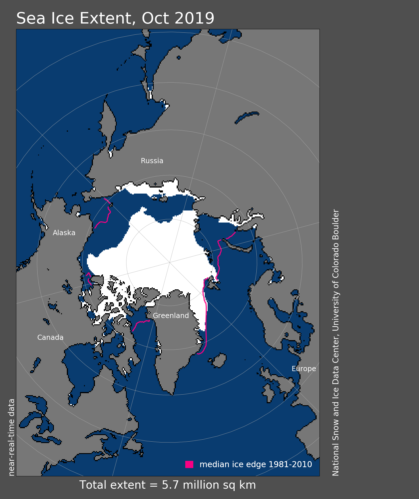
Figure 1. Arctic sea ice extent for October 2019 was 5.67 million square kilometers (2.19 million square miles). The magenta line shows the 1981 to 2010 average extent for that month. Sea Ice Index data. About the data
Credit: National Snow and Ice Data Center
High-resolution image
Arctic sea ice extent averaged for October 2019 was 5.66 million square kilometers (2.19 million square miles), the lowest in the 41-year continuous satellite record. This was 230,000 square kilometers (88,800 square miles) below that observed in 2012—the previous record low for the month—and 2.69 million square kilometers (1.04 million square miles) below the 1981 to 2010 average. Daily ice extent began tracking below 2012 levels on October 13 and continued to do so through the end of the month, which was enough to reach a new record monthly low at 5.66 million square kilometers (2.19 million square miles). The Arctic gained only 2.79 million square kilometers (1.08 million square miles) of ice in October 2019, compared to 3.81 million square kilometers (1.47 million square miles) in October 2012.
Autumn freeze up was slow during the first half of October, with most of the increases in the eastern Beaufort Sea and Laptev Sea. During the second half of the month, ice began to grow quickly along the coastal regions of the East Siberian and Laptev Seas. Sea ice also began forming around northern to north-eastern Svalbard. Overall, the ice edge remained considerably north of its average location throughout the Beaufort, Chukchi, Kara, and Barents Seas, as well as within Baffin Bay. However, around Svalbard, the sea ice has returned to near average conditions for this time of year. As of October 15, the ice extent in the Chukchi Sea is the lowest on record for this time of year.
Conditions in context
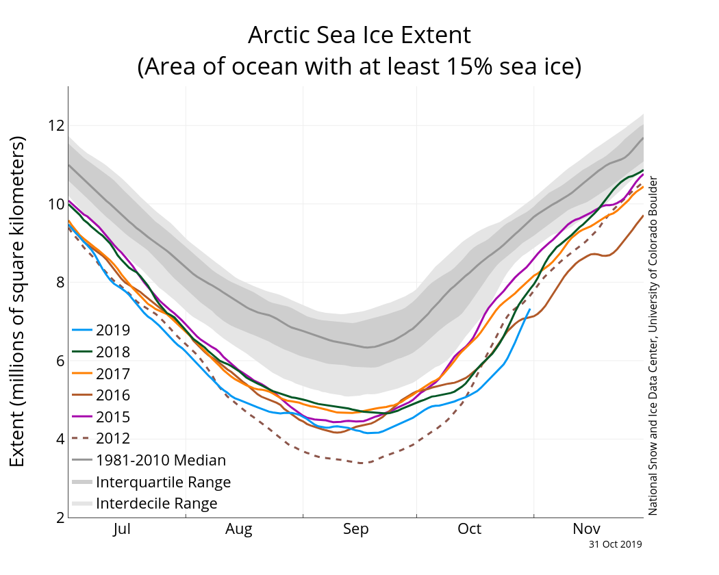
Figure 2a. The graph above shows Arctic sea ice extent as of October 31, 2019, along with daily ice extent data for four previous years and the record low year. 2019 is shown in blue, 2018 in green, 2017 in orange, 2016 in brown, 2015 in purple, and 2012 in dotted brown. The 1981 to 2010 median is in dark gray. The gray areas around the median line show the interquartile and interdecile ranges of the data. Sea Ice Index data.
Credit: National Snow and Ice Data Center
High-resolution image
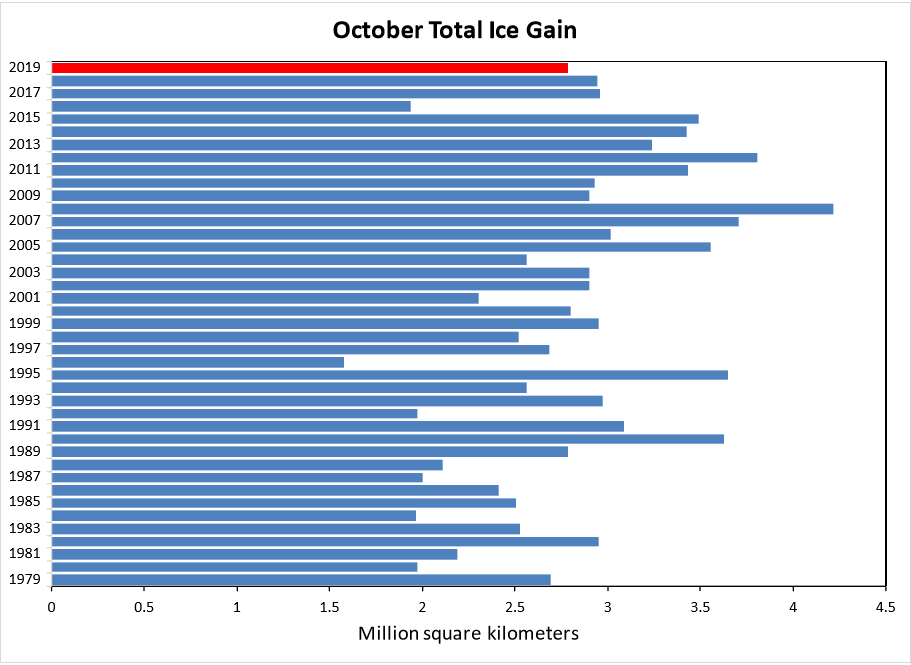
Figure 2b. The chart above shows October sea ice gain in millions of square kilometers from 1979 to 2019, with 2019 shown in red and the climatological average ice growth in gray. October 2019 ice gain was close to average.
Credit: National Snow and Ice Data Center
High-resolution image
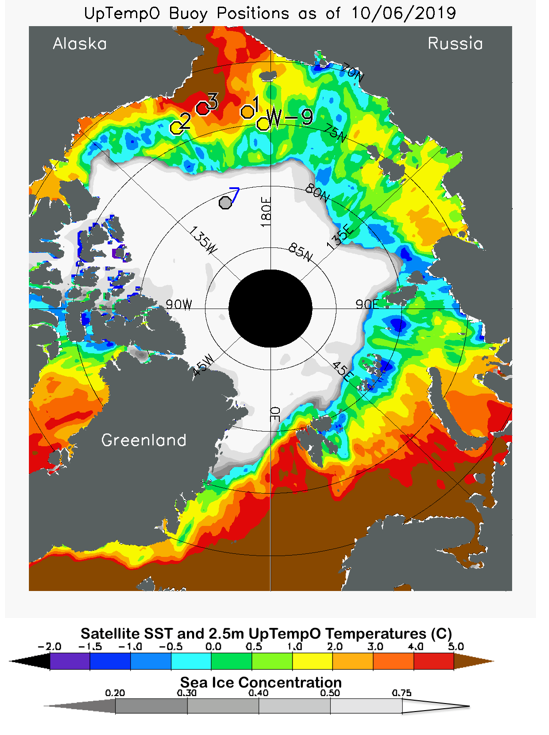
Figure 2c. This map shows satellite-derived sea surface temperature (SST) and temperatures at the Upper layer Temperature of the Polar Oceans (UpTempO) buoys, along with sea ice concentration. UpTempO buoys measure ocean temperature in the euphotic surface layer of the Polar Oceans.
Credit: University of Washington
High-resolution image

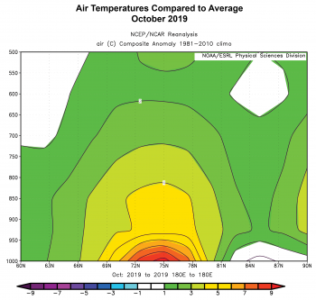
Figure 2d. This figure shows air temperatures compared to average for October 2019. This is a cross section (latitude by height, up to the 500 hPa level) along the 180 degrees E meridian, which is the date line and cuts through the Chukchi Sea. The prominent area in red at and near the surface manifests the extensive open water in the Chukchi Sea.
Credit: NOAA/ESRL Physical Sciences Division.
High-resolution image
Ice growth through October 2019 averaged 89,900 square kilometers (34,700 square miles) per day. This was similar to the average rate of ice growth in October of 89,100 square kilometers (34,400 square miles) per day. However, the growth rate varied greatly during the month. On October 1, extent tracked 682,000 square kilometers (263,000 square miles) above that for the same day in 2012. However, ice growth was slow, and by October 13, extent began tracking below 2012, setting new record daily lows during the latter half of the month. On October 18, extent was 3.08 million square kilometers (1.19 million square miles) below the 1981 to 2010 average, the largest daily departure from average observed in the satellite data record. Ice growth rates increased during the last two weeks of the month so that by October 30, the extent started tracking above that recorded in 2016.
Overall, sea ice extent increased 2.79 million square kilometers (1.08 square miles) in October 2019. The largest October ice gain was in 2008 (4.22 million square kilometers; 1.63 million square miles), followed closely by 2012 (3.81 million square kilometers; 1.47 million square miles) and 2007 (3.70 million square kilometers; 1.43 million square miles) (Figure2b). However, this October, sea surface temperatures remained relatively high (2 to 5 degrees Celsius; 36 to 41 degrees Fahrenheit) in early October throughout large areas of the Chukchi, Laptev, Kara, and Barents Seas (Figure 2c). High sea surface temperatures imply considerable heat storage in the ocean surface layer, consistent with delayed freeze up in those regions.
Air temperatures at 925 hPa level (about 2,500 feet above the surface) for the month were 1 to 4 degrees Celsius (2 to 7 degrees Fahrenheit) above average over most of the Arctic Ocean, with temperatures north of Greenland reaching 7 degrees Celsius (13 degrees Fahrenheit) above the 1981 to 2010 average. Below average air temperatures were only found southeast of Svalbard (on the order of 1 to 2 degrees Celsius, or 2 to 4 degrees Fahrenheit). Of particular interest are the unusually high temperatures at and near the surface in the Beaufort and Chukchi Seas due to the extensive open water there. These manifest large energy fluxes from the ocean to the atmosphere, as the warm ocean water cools to the freezing point. The vertical cross section (latitude by height) of air temperatures expressed as departures from average along the 180oE meridian (the date line, which cuts through the Chukchi Sea) shows this effect clearly (Figure 2d). Unusually high temperatures in the Beaufort and Chukchi Seas will linger until the ocean surface freezes over.
October 2019 compared to previous years
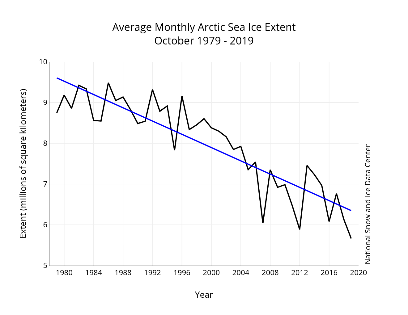
Figure 3. Monthly October ice extent for 1979 to 2019 shows a decline of 9.8 percent per decade.
Credit: National Snow and Ice Data Center
High-resolution image
Monthly sea ice extent reached a record low in October as assessed over the period of satellite observations. The linear rate of sea ice decline for October is 81,400 square kilometers (31,400 square miles) per year, or 9.8 percent per decade relative to the 1981 to 2010 average.
Ice returns to “normal” near Svalbard
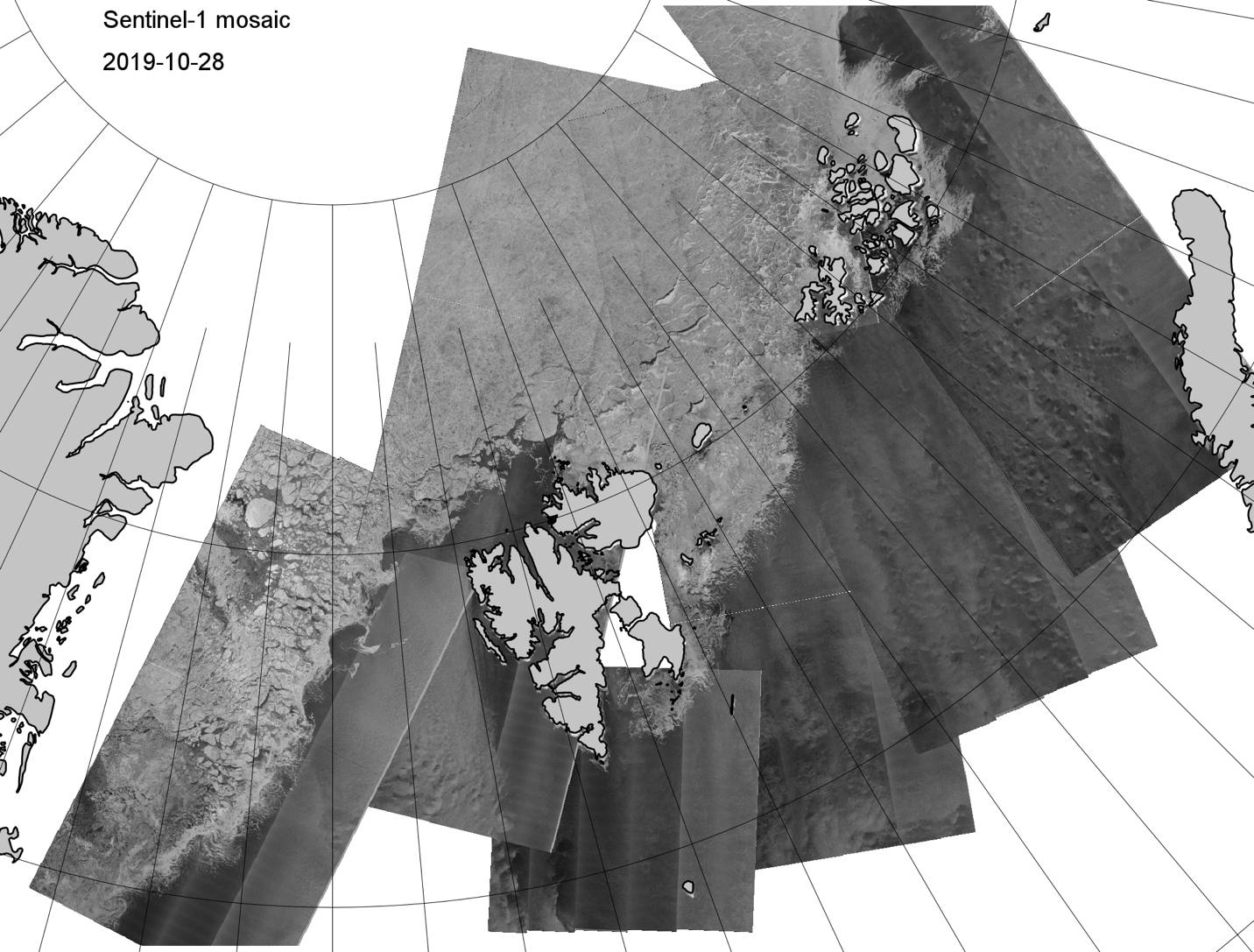
Figure 4. Sea ice extent around Svalbard has returned to the 1981 to 2010 median position for this time of year, as shown by the Synthetic Aperture Radar (SAR) data from the Sentinel-1 mission for October 28, 2019.
Credit: Norwegian Meteorological Institute
High-resolution image
Recent winters have seen unusually low ice extent in the Barents Sea. Several studies have demonstrated a link between reduced winter ice in this region and increased ocean heat transport from the north Atlantic that prevents ice formation. However, the ocean heat transport is variable, and weakening could allow for temporary recovery of winter ice conditions in this region despite a warming climate. This appears to have been the case last winter, when the ice edge in the Barents Sea returned to its 1981 to 2010 average position. Early evidence suggests that this recovery may continue into the coming winter. Synthetic Aperture Radar (SAR) data from the Sentinel-1 mission for October 28 (Figure 4) shows the ice extent around Svalbard has returned to the 1981 to 2010 median position for this time of year. However, extent still remains much below average over most of the northern Barents Sea.
Update on sea ice age
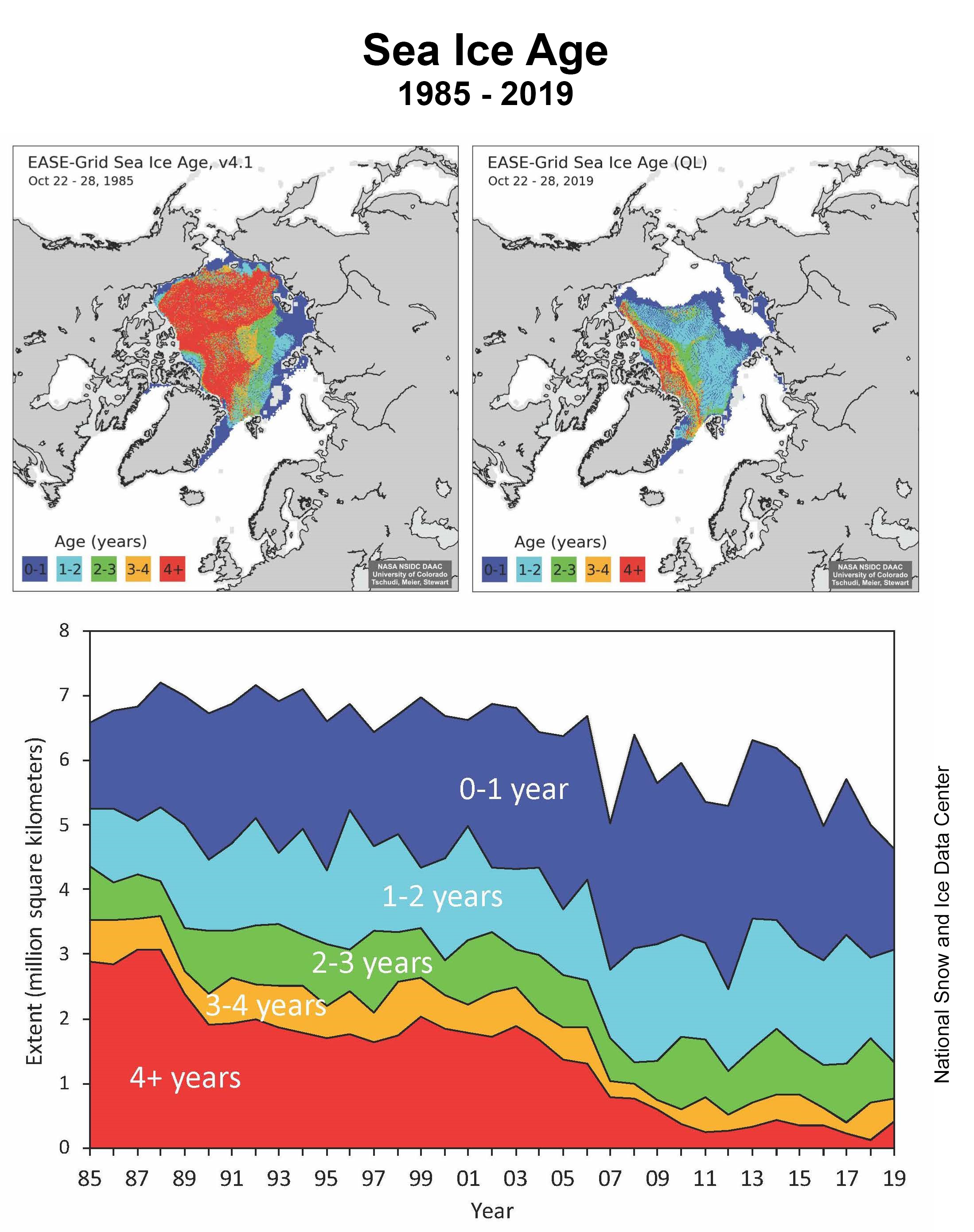
Figure 5. The top left map shows sea ice age for October 22 to 28, 1985 while the right map shows the same week in 2019. The bottom graph shows a time series of ages for that week from 1985 to 2019 from the NSIDC EASE-Grid Sea Ice Age, Version 4.
Credit: National Snow and Ice Data Center
High-resolution image
After the sea ice minimum in September, the remaining sea ice had its “birthday,” aging one year in the NSIDC sea ice age fields. Much of the Arctic is now covered by second-year (1- to 2-year-old) ice, meaning ice that grew over the 2018 autumn and 2019 winter and survived the melt season. There is also already about 1 million square kilometers (386,100 square miles) of ice that has grown since the September 2019 minimum—the 0- to 1-year-old category—but there is substantially less ice older than two years than there used be—about one-third of the amount “old ice” as there was in the mid-1980s and about one-half as much as there was as recently as the mid-2000s.
IPCC Special Report on the Ocean and Cryosphere in a Changing Climate (SROCC)
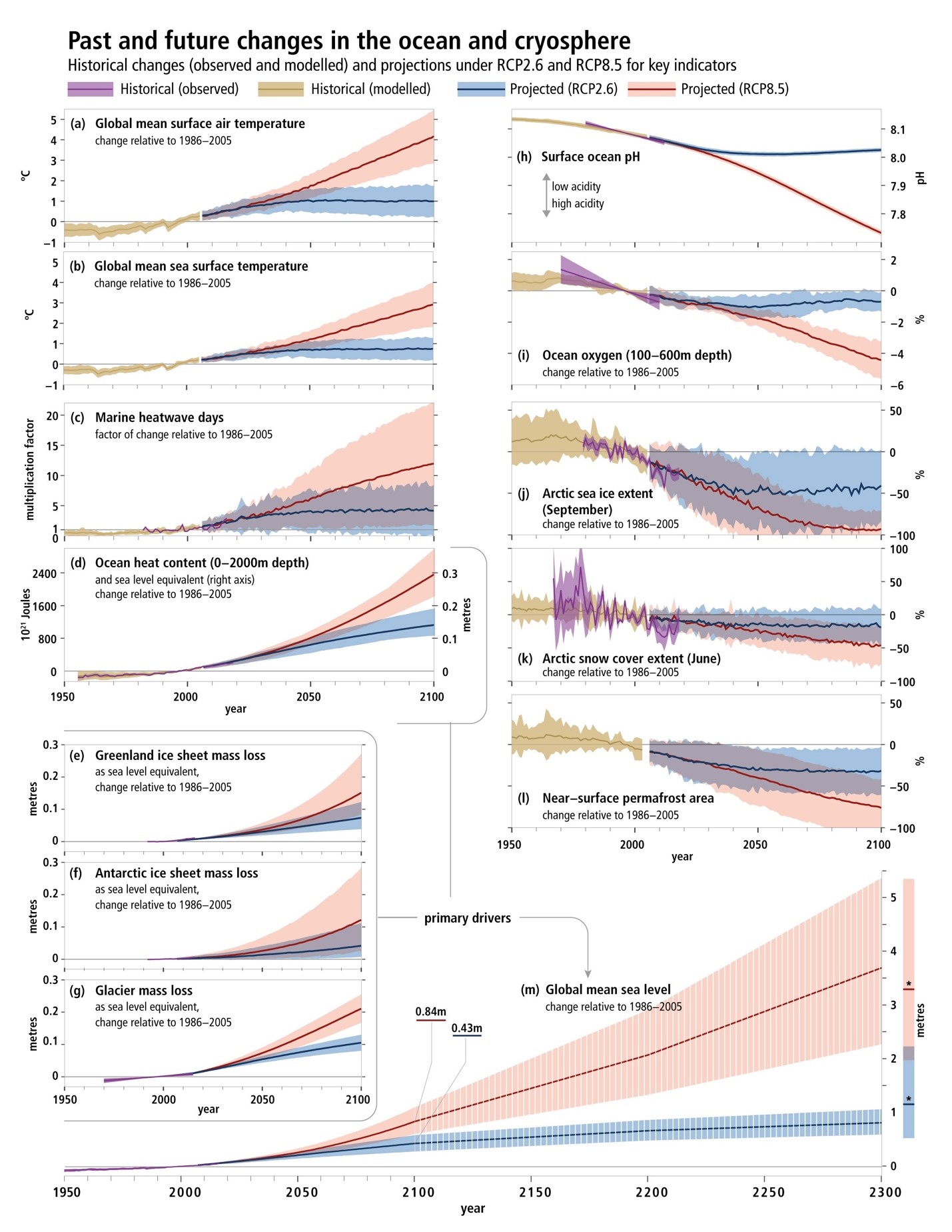
Figure 6. The Intergovernmental Panel on Climate Change (IPCC) Special Report on the Ocean and Cryosphere in a Changing Climate (SROCC) Summary for Policymakers shows the observed and modeled historical changes in the ocean and cryosphere since 1950, as well as the future projections under a low emission scenario that limits the global warming to less than 2 degrees Celsius (4 degrees Fahrenheit), compared to a high emission scenario where global temperatures rise above 4 degrees Celsius (7 degrees Fahrenheit). Changes are shown relative to 1986 to 2005 for: (a) global mean surface air temperature; (b) global-mean sea surface temperature; (c) number of surface ocean marine heatwave days; (d) global ocean heat content (0 to 2000 meter depth); (e) Greenland mass loss; (f) Antarctic mass loss; (g) glacier mass loss; (h) global mean surface pH; (i) global mean ocean oxygen averaged over 100 to 600 meter depth; (j) Arctic sea ice; (k) Arctic snow cover; (l) near-surface permafrost area and (m) global sea level.
Credit: International Panel on Climate Change (IPCC)
High-resolution image
In late September, the Intergovernmental Panel on Climate Change (IPCC) released a new report on the state of the oceans and the cryosphere, highlighting observed changes and forecasts of what may occur in the future. The report provides a timely update on how the cryosphere is changing and its implications for society and ecosystems. It also highlights the high confidence in rates of Arctic sea ice loss and its causes, with anthropogenic forcing and natural climate variability playing nearly equal roles.
NSIDC scientist Julienne Stroeve was one of the contributors to the chapters on sea ice and Arctic amplification—the outsized rise in Arctic air temperatures compared to the globe as a whole. One of the drivers of the special report is recognition that the oceans play a key role in the changing climate system, absorbing 90 percent of the excess heat within Earth’s system and up to a third of the carbon dioxide. Sea ice also reflects much of the sun’s energy back out to space, helping to keep the planet cooler than it otherwise would be. There is high confidence that the Arctic sea ice cover will continue to shrink (Figure 6).
The effects of anthropogenic warming are not as clear in the Antarctic, in particular for sea ice trends. This results in low confidence in any forecast of how Antarctic sea ice will evolve. The report also highlights how permafrost and snow cover are expected to change, as well as sea level rise from glacier and ice sheet mass losses. Given that the Antarctic ice sheet is starting to contribute more each year to global mean sea level rise, the potential for a meter (3.28 feet) of sea level rise by the end of the century remains possible. A key message of the report is that limiting global warming to a total of less than 2 degrees Celsius (4 degrees Fahrenheit) by the end of the century will help to mitigate the negative effects of climate change.

