Updating the sea ice baseline

This July, NSIDC plans to change the baseline climatological period for Arctic Sea Ice News and Analysis and the Sea Ice Index, the data set we use for our sea ice analysis. We are making this change to match the comparison time frames used by other climate research.

Until now, we have used the 22-year period 1979 to 2000 when comparing current sea ice extent to past conditions. When NSIDC first began to monitor and analyze sea ice extent, a longer period was not available. Since the satellite record is now extended, we are choosing to move to a more standard 30-year reference period, from 1981 to 2010.

A 30-year period typically defines a climatology (comparsion period) and is the standard used by organizations such as the World Meteorological Organization (WMO) and the U.S. National Oceanic and Atmospheric Administration (NOAA). Thirty years is considered long enough to average out most variability from year to year, but short enough so that longer-term climate trends are not obscured.

These maxims about climate averages come from the world of weather and climate. Sea ice responds to changes in energy or heat differently from other systems on Earth. So the assumptions behind the use of 30-year averages for weather may not hold true for sea ice, particularly in light of the rapid decrease and repeated record low minimum extents in the Arctic during the past decade. However, matching the 1981 to 2010 period brings us in line with other climate research.

The monthly and daily sea ice extent images and data values will not change, but data and images that are based on the average or median will change. For example, the trend plot for sea ice extent will have a different scale, and the value of the slope, expressed as change in percent per decade, will change, because this value is relative to the average period. On the the monthly and daily extent images, the position of the average extent lines will change.

In our July analysis, we will provide more information to help readers put these changes into the larger context of changing climate and changing ice.

Un-baked Alaska

Arctic sea ice extent declined at a near-average rate through May, but overall it remained below average compared to the 1979 to 2000 average. The Arctic Oscillation (AO) varied through the month between modest positive and negative phases. Winds from the north and northwest and persistent snow cover over central Alaska made much of the month unusually cold there. The last part of the month saw much higher temperatures.

Overview of conditions

Figure 1. Arctic sea ice extent for May 2013 was 13.10 million square kilometers (5.05 million square miles). The magenta line shows the 1979 to 2000 median extent for that month. The black cross indicates the geographic North Pole.  Sea Ice Index data. About the data||Credit: National Snow and Ice Data Center|High-resolution image

Figure 1. Arctic sea ice extent for May 2013 was 13.10 million square kilometers (5.06 million square miles). The magenta line shows the 1979 to 2000 median extent for that month. The black cross indicates the geographic North Pole. Sea Ice Index data. About the data

Credit: National Snow and Ice Data Center
High-resolution image

Sea ice extent in May 2013 averaged 13.10 million square kilometers (5.06 million square miles). This is 500,000 square kilometers (193,000 square miles) below the 1979 to 2000 average for the month. As has been the case for the past several years, ice extent was below average in the Barents Sea on the Atlantic side of the Arctic. Greater than average ice extent prevailed on the Pacific side of the Arctic in the Bering Sea and Sea of Okhotsk.

Conditions in context

Time series graph as of June 14, 2013

Figure 2. The graph above shows Arctic sea ice extent as of June 2, 2013, along with daily ice extent data for five previous years. 2013 is shown in blue, 2012 in green, 2011 in orange, 2010 in pink, 2009 in navy, and 2008 in purple. The 1979 to 2000 average is in dark gray. The gray area around this average line shows the two standard deviation range of the data. Note: 2011 was inadvertently omitted from this graph; corrected June 17. Sea Ice Index data.

Credit: National Snow and Ice Data. High resolution image

The AO varied through the month between modest positive and negative phases. However, May was characterized by a broad region of unusually low pressure covering much of the western Arctic, namely the Beaufort, Chukchi, and East Siberian seas. Earlier large-scale fracturing of the sea ice off the northeast coast of Alaska and north of the Canadian Archipelago mentioned in our past post was linked to a pattern of high pressure over the Arctic and a strongly negative phase of the AO.

There are several open water areas, or polynyas, along the Arctic coast, as is typical for this time of year. Small patches of open water are present along the Laptev Sea coast north of Russia, and at the northern end of Baffin Bay. These will expand as summer melting and warmer conditions progress in the Arctic.

May 2013 compared to previous years

Figure 3. Monthly May ice extent for 1979 to 2013 shows a decline of 2.24% per decade.||Credit: National Snow and Ice Data Center |High-resolution image

Figure 3. Monthly May ice extent for 1979 to 2013 shows a decline of -2.24 percent per decade.

Credit: National Snow and Ice Data Center
High-resolution image

May 2013 was the tenth lowest May in the satellite record, 390,000 square kilometers (151,000 square miles) above the record low of 12.58 million square kilometers (4.86 million square kilometers) in 2004.*

Through the month of May this year, extent declined at an average rate of 36,400 square kilometers (14,100 square miles) per day, slower than the 1979 to 2000 average of 44,100 square kilometers (17,000 square miles) per day.

*Note: We originally stated that the record low had occurred in May 2011. After reviewing the data, we corrected this statement. See the Sea Ice Index for data on past May ice extent.

Snow cover update

Figure 4. This snow cover anomaly map shows the difference between snow cover for May 2013, compared with average snow cover for May from 1971 to 2000. Areas in orange and red indicate lower than usual snow cover, while regions in blue had more snow than normal. |Credit: National Snow and Ice Data Center, data courtesy Rutgers University Global Snow Lab  High-resolution image

Figure 4. This snow cover anomaly map shows the difference between snow cover for May 2013, compared with average snow cover for May from 1971 to 2000. Areas in orange and red indicate lower than usual snow cover, while regions in blue had more snow than normal.

Credit: National Snow and Ice Data Center, courtesy Rutgers University Global Snow Lab
High-resolution image

Monthly snow cover anomaly data from the Rutgers University Global Snow Lab  show that snow cover for the month of May was significantly low in eastern Siberia, northern Europe, and the Rocky Mountains in North America. Data also show a few greater-than-average regions in Alaska—contributing to the lower temperatures there—and on  the Tibetan Plateau.

Weekly and daily data from the Global Snow Lab show that May began with greater-than-average snow cover in Tibet and the Great Plains of Canada and the United States. By the end of the month, however, snow extent was near average to lower than average throughout the Northern Hemisphere, and much lower than average in northeastern Siberia. Overall, snow cover in May 2013 was the lowest on record in forty-seven years of data for Eurasia, and third lowest overall for the Northern Hemisphere, trailing only 2012 and 2010.

Chilly in Alaska

Figure 5. This image shows air temperature anomalies at the 925 hPa level averaged for May 2013, compared to averages over the period 1981 to 2010. Temperatures were lower than average over Alaska, while temperatures across much of Siberia were above average. ||Credit: NSIDC courtesy NOAA/ESRL PSDHigh-resolution image

Figure 5. This image shows air temperature anomalies at the 925 hPa level averaged for May 2013, compared to averages over the period 1981 to 2010. Temperatures were lower than average over Alaska, while temperatures across much of Siberia were above average.

Credit: NSIDC courtesy NOAA Earth System Research Laboratory Physical Sciences Division
High-resolution image

Lower than average temperatures were the rule this past month for both Greenland and Alaska, while temperatures across much of Siberia were above average. Temperatures over central Alaska at the 925 hPa level were 4 to 5 degrees Celsius (7 to 9 degrees Fahrenheit) colder than usual, making this one of the coldest springs on record for cities like Fairbanks. These low temperatures can be linked to winds from the north and northwest over central Alaska and persistent snow cover. However, the end of the month saw much higher temperatures, reaching more than 80 degrees Fahrenheit (27 degrees Celsius) in Fairbanks.

Because of the low temperatures, ice on the Tanana River, which runs through Fairbanks, Alaska, broke up on May 20 at 2:41 p.m.—the latest date and time on a record which extends for nearly a century. Ice break-up has been carefully recorded at the town of Nenana, about 70 kilometers (44 miles) downstream on the Tanana River from Fairbanks, by timing the tipping of a large tripod erected on the river ice. This is a matter of some importance for Alaskans, as there is a large statewide lottery based on picking the exact time of ice break-up. In most years, winning this lottery requires picking the time to the precise minute of tipping. Congratulations to Warren and Yvonne Snow, for your excellent climate forecasting (and on having a wonderful last name)!


April on average

Arctic sea ice extent declined at an approximately average rate through April. While the Arctic Oscillation was in its negative phase for most of winter, in mid April it turned positive. This helped to bring in warm air over Eurasia, although air temperatures over the sea ice cover remain below freezing.

Overview of conditions

Figure 1. Arctic sea ice extent for April 2013 was X.XX million square kilometers (X.XX million square miles). The magenta line shows the 1979 to 2000 median extent for that month. The black cross indicates the geographic North Pole.  Sea Ice Index data. About the data||Credit: National Snow and Ice Data Center|High-resolution image

Figure 1. Arctic sea ice extent for April 2013 was 14.37 million square kilometers (5.54 million square miles). The magenta line shows the 1979 to 2000 median extent for that month. The black cross indicates the geographic North Pole. Sea Ice Index data. About the data

Credit: National Snow and Ice Data Center
High-resolution image

Sea ice extent averaged for the month of April 2013 was 14.37 million square kilometers (5.54 million square miles). This is 630,000 square kilometers (243,000 square miles) below the 1979 to 2000 average for the month, and is the seventh-lowest April extent in the satellite record.

In the earlier part of the satellite data record, average April extent remained above 15 million square kilometers (5.8 million square miles). Since 1989 the extent has mostly remained between 14 and 15 million square kilometers (5.4 and 5.8 million square miles). The years 1993 and 1999 were exceptions, when extent exceeded 15 million square kilometers (5.8 million square miles), as well as 2006 and 2007, when extent dropped below 14 million square kilometers (5.4 million square miles).

A large area of open water has started to form around Franz Josef Land and north of Svalbard. Polynyas are also appearing in the Kara and East Siberian seas.

The walrus and whaling season has begun in Arctic Alaska. The Study of Environmental Arctic Change (SEARCH) Sea Ice for Walrus Outlook (SIWO) is now providing weekly sea ice outlooks as a resource for Alaska Native subsistence hunters, coastal communities, and others interested in sea ice and walrus or whales. With spring sea ice conditions being thinner and less predictable than in the past due to warming in the Arctic, the sea ice outlook helps hunters plan their activities.

Conditions in context

Figure 2. The graph above shows Arctic sea ice extent as of April 30, 2013, along with daily ice extent data for five previous years. 2013 is shown in blue, 2012 in green, 2011 in orange, 2010 in pink, 2009 in navy, and 2008 in purple. The 1979 to 2000 average is in dark gray. The gray area around the average line shows the two standard deviation range of the data. Sea Ice Index data.||Credit: National Snow and Ice Data Center|High-resolution image

Figure 2. The graph above shows Arctic sea ice extent as of April 30, 2013, along with daily ice extent data for five previous years. 2013 is shown in blue, 2012 in green, 2011 in orange, 2010 in pink, 2009 in navy, and 2008 in purple. The 1979 to 2000 average is in dark gray. The gray area around the average line shows the two standard deviation range of the data. Note: 2011 was inadvertently omitted from this graph; corrected June 17. Sea Ice Index data.

Credit: National Snow and Ice Data Center
High-resolution image

Through the month of April, the Arctic lost 1.5 million square kilometers of ice (444,000 square miles), which is slightly higher than the average for the month. Air temperatures at the 925 hPa level (approximately 3,000 feet above sea level) in April were 5 to 7 degrees Celsius (9 to 13 degrees Fahrenheit) higher than average in the East Siberian Sea and 3 to 5 degrees Celsius (5 to 9 degress Fahrenheit) higher than average in the Kara Sea. Temperatures were 3 to 5 degrees Celsius (5 to 9 degrees Fahrenheit) below average over Alaska. The dominant feature of the Arctic sea level pressure field for April 2013 was unusually high pressure over Alaska and Siberia and below average pressure over the Kara and Barents seas.  During the middle of the month, the Arctic Oscillation switched from a negative to a positive phase, with anomalously high sea level pressure over Alaska combined with below average pressure over Greenland and the North Atlantic. This brought in warm air over Eurasia, and above average air temperatures throughout the eastern Arctic.

The reductions in April ice extent this year and over the satellite record are predominantly due to reduced ice cover in the Kara and Barents seas. In contrast, ice extent continues to remain slightly above normal in the Bering Sea.

April 2013 compared to previous years

Figure 3. Monthly April ice extent for 1979 to 2013 shows a decline of -2.3% per decade.

Credit: National Snow and Ice Data Center
High-resolution image

Average Arctic sea ice extent for April 2013 was the seventh lowest for the month in the satellite record. Through 2013, the linear rate of decline for April ice extent is -2.3 percent per decade relative to the 1979 to 2000 average.

IceBridge Arctic flights

Figure 4. This chart shows the flight tracks of IceBridge P-3 aircraft flights over the Arctic through April 26, 2013.

Credit: NASA Operation IceBridge
High-resolution image

On 20 March 2013, NASA resumed Operation IceBridge aircraft missions over the Arctic. The IceBridge mission was initiated in 2009 to collect airborne measurements of sea ice and ice sheet thickness, to bridge the gap between NASA’s Ice, Cloud and Land Elevation Satellite (ICESat) and the upcoming ICESat-2 mission. This spring, areas not extensively covered in previous campaigns were a focus as well as flight tracks corresponding to the European CryoSat-2 satellite. Several successful flights were flown across the Beaufort and Chukchi seas in March and early April while the aircraft was stationed in Fairbanks, Alaska and Greenland’s Thule Air Base. Afterwards NASA’s P-3B aircraft was moved to Kangerlussuaq, Greenland for flights over the ice sheet. Towards the end of April, the aircraft was once again stationed in Thule, allowing additional ice sheet flights over the north central part of Greenland ice sheet and the resumption of sea ice flights over large portions of Arctic sea ice. The latter included a repeat of a 2012 flight line aimed at sampling a large region of the Canada Basin. This year’s Arctic IceBridge mission ended on 2 May, with the successful completion of ten sea ice and fifteen ice sheet flights.

Earliest satellite maps of Antarctic and Arctic sea ice

Figure 5. The National Snow and Ice Data Center scanned close to 40,000 images from Nimbus 1 satellite data to produce the earliest satellite images of Arctic and Antarctic satellite extent. The left image is a composite of the Arctic and the right image is a composite of the Antarctic.

Credit: NSIDC
High-resolution image

While the modern satellite data record for sea ice begins in late 1978, some data are available from earlier satellite programs. NSIDC has been involved in a project to map sea ice extent using visible and infrared band data from NASA’s Nimbus 1, 2, and 3 spacecraft, which were launched in 1964, 1966, and 1969. Analysis of the Nimbus data has revealed Antarctic sea ice extents that are significantly larger and smaller than seen in the modern 1979 to 2012 satellite passive microwave record. The September 1964 average ice extent for the Antarctic is 19.7 ± 0.3 million square kilometers (7.6 million ± 0.1 square miles. This is more than 250,000 square kilometers (97,000 square miles) greater than the 19.44 million square kilometers (7.51 million square miles) seen in 2012, the record maximum in the modern data record. However, in August 1966 the maximum sea ice extent fell to 15.9 ± 0.3 million square kilometers (6.1 ± 0.1 million square miles). This is more than 1.5 million square kilometers (579,000 square miles) below the passive microwave record low September of 17.5 million square kilometers (6.76 million square miles) set in 1986.

The early satellite data also reveal that September sea ice extent in the Arctic was broadly similar to the 1979 to 2000 average, at 6.9 million square kilometers (2.7 million square miles) versus the average of 7.04 million square kilometers (2.72 million square miles).

In memoriam

We dedicate this post to Dr. Katharine Giles, who was tragically killed cycling to work on 8 April 2013. Together with Dr. Laxon, Katherine Giles worked to retrieve sea ice thickness from satellite radar altimeter data. In 2007 she was the first to show that this data could also be used to show how winds affect the newly exposed Arctic Ocean. Since Dr. Laxon’s death earlier this year, Katharine worked hard to continue his legacy and supervise his students. We have lost yet another talented scientist and a great friend.

Reference

Meier, W. N., D. Gallaher, and G. C. Campbell. 2013. New estimates of Arctic and Antarctic sea ice extent during September 1964 from recovered Nimbus I satellite imagery. The Cryosphere, 7, 699–705, doi:10.5194/tc-7-699-2013.

Spring has sprung in the Arctic

Arctic sea ice has passed its annual maximum extent and is beginning its seasonal decline through the spring and summer. While total extent was not at record low, it remained well below average through March. Ice fracturing continued north of Alaska, and the Arctic Oscillation was in a strongly negative phase during the second half of the month, with unusually high sea level pressure over almost all of the Arctic Ocean. Levels of multiyear ice remain extremely low. The ice is thinner, and satellite data suggests that first-year ice may now cover the North Pole area for the first time since winter 2008.

Overview of conditions

Figure 1. Arctic sea ice extent for March 2013 was 15.04 million square kilometers (5.81 million square miles). The magenta line shows the 1979 to 2000 median extent for that month. The black cross indicates the geographic North Pole. Sea Ice Index data. About the data

Credit: National Snow and Ice Data Center
High-resolution image

Arctic sea ice extent in March 2013 averaged 15.04 million square kilometers (5.81 million square miles). This is 710,000 kilometers (274,000 square miles) below the 1979 to 2000 average extent, and 610,000 square kilometers (236,000 square miles) above the record low for the month, which happened in 2006. Continuing a trend in recent winters, ice extent was near or below average levels throughout most of the Arctic, with the exception of higher extent in the Bering Sea.

Conditions in context

Figure 2. The graph above shows Arctic sea ice extent as of April 1, 2013, along with daily ice extent data for the previous five years. 2012 to 2013 is shown in blue, 2011 to 2012 in green, 2010 to 2011 in pink, 2009 to 2010 in navy, and 2008 to 2009 in purple. The 1979 to 2000 average is in dark gray. The gray area around this average line shows the two standard deviation range of the data. Sea Ice Index data.

Credit: National Snow and Ice Data Center
High-resolution image

As Arctic sea ice reaches its maximum extent in March, the net gain or loss through the month tends to be small. This year, extent decreased 5,400 square kilometers (2,100 square miles) between the beginning and end of the month, with the decline in the second half of the month slightly outweighing the increase over the first half. Air temperatures (at the 925 mb level, or about 3,000 feet) were 3 to 6 degrees Celsius (5 to 11 degrees Fahrenheit) higher than average over the central Arctic Ocean, with cooler conditions compared to average (3 to 6 degrees Celsius, or 5 to 11 degrees Fahrenheit) over the Kara and Barents seas.

The circulation pattern known as the Arctic Oscillation (AO) reached an extreme negative phase in the second half of the month, associated with unusually high sea level pressure covering nearly the entire Arctic Ocean. The AO index , a measure of the state of the atmosphere over the Arctic, fell to as low as -5 sigma in mid March. This caps several months of a persistently negative AO. In the past, a negative AO in winter has been associated with the retention of thick ice in the Arctic Ocean and reduced export by drift into the Atlantic, favoring more extensive sea ice at the end of the summer melt season. However, in recent years, this relationship has not held and low summer extents have followed winters with strong negative AO. The month was also notable for continued fracturing of the ice cover in the Beaufort and Chukchi seas north of Alaska, as seen in a new animation by the NASA Earth Observatory . This is consistent with wind patterns associated with the strong negative pattern of the AO.

March 2013 compared to previous years

Figure 3. Monthly March ice extent for 1979 to 2013 shows a decline of 2.5% per decade.

Credit: National Snow and Ice Data Center
High-resolution image

Average ice extent for March 2013 was the fifth lowest for the month in the satellite record. Through 2013, the linear rate of decline for March ice extent is 2.5% per decade relative to the 1979 to 2000 average. While the percentage trend is lower than in the summer, the average rate of decrease is 39,800 square kilometers (15,300 square miles) per year, roughly the size of Maryland and Delaware combined.

A record extent of first-year ice in the Arctic

Figure 4. Imagery from the European Advanced Scatterometer (ASCAT) for December 2, 2012 (top) and March 28, 2013 (bottom) show the change in multiyear ice coverage over the winter season, as outlined by the colored lines. In winter, multiyear ice changes are due to the motion of the ice, either export through Fram Strait or redistribution within the Arctic Ocean.

Credit: Advanced Scatterometer imagery courtesy NOAA NESDIS, analysis courtesy T. Wohlleben, Canadian Ice Service
High-resolution image

Between the 2012 summer minimum and the 2013 winter maximum, sea ice extent increased 11.72 million square kilometers (4.53 million square miles), the largest increase in the satellite record. This was primarily due to the extreme record low ice extent in September 2012, which resulted in a near-record high first-year ice extent. This is evident in imagery from the Advanced Scatterometer (ASCAT) sensor on the European METOP-A satellite provided by National Oceanic and Atmospheric Administration’s National Environmental Satellite, Data, and Information Service (NOAA NESDIS). Analysis by Trudy Wohlleben at Environment Canada indicates that multiyear ice is relegated to areas far from the Alaskan and Eurasian coasts. Over the winter, some multiyear ice recirculated into the Beaufort Sea where significant melt of multiyear ice has occurred in recent summers. Also, some multiyear ice has been lost, as it moved out of the Arctic through Fram Strait. The boundary between primarily first-year ice and multiyear ice is now near the North Pole (indicated by the small black circle near the center of the image), marking the first time since the winter of 2008 that a substantial amount of first-year ice may be covering the pole as we enter the melt season.

Oldest ice continues to decline

Figure 5. The map at top shows the ages of ice in the Arctic at the end of March 2013; the bottom graph shows how the percentage of ice in each age group has changed from 1983 to 2013.

Credit: NSIDC courtesy J. Maslanik and M. Tschudi, University of Colorado
High-resolution image

While multiyear ice used to cover up to 60% of the Arctic Ocean, it now covers only 30%. There is a slight rebound in the oldest ice (4+ years old), a remnant of the large amount of first-year ice that formed during the winter after the 2007 record minimum. However, most of that new ice has not survived through the subsequent years. The oldest ice now comprises only 5% of the ice in the Arctic Ocean. This is a slight uptick from last winter’s record low of 3%, but still far less than during the 1980s when old ice covered roughly 25% of the region.

 Satellite estimates show continued thinning

Figure 6. Estimates of February/March average sea ice thickness for 2004 to 2008 from NASA’s ICESat (left) and February/March 2012 from CryoSat-2 (right). Colors indicate ice thickness in meters, with blue indicating 1-meter thick sea ice and red indicating 5-meter thick sea ice. The black and gray lines in the CryoSat-2 image are tracks of airborne data collected for validation. The triangle, circle, and square are locations of upward-looking sonar (ULS) moorings, also used for validation of the CryoSat-2 estimates.

Credit: American Geophysical Union
High-resolution image

The ASCAT data and ice age data both suggest a continued thinning of the ice pack, and overall decline in its volume, but they do not provide direct information on ice thickness. However, the European Space Agency’s CryoSat-2 satellite, launched in April 2010, now provides estimates of sea ice thickness distribution across the Arctic Ocean. A new paper by Laxon et al. (2013) shows the first published results from CryoSat-2 and compares them with thickness estimates from NASA’s ICESat satellite, which operated from 2003 to 2009. The CryoSat-2 results indicate continued thinning since 2008. Significantly, ice along the north coast of Greenland appears to have thinned—in the past this has been the site of some of the thickest sea ice in the Arctic. The paper also shows that total volume estimates from CryoSat-2 agree well with University of Washington’s Pan-Arctic Ice Ocean Modeling and Assimilation System (PIOMAS)  estimates.

In memoriam

We dedicate this post to Seymour Laxon, who tragically passed away in early January. Laxon was a driving force behind the CryoSat-2 mission, a leading innovator in the development of sea ice altimetry, an outstanding scientist, and a great friend to the sea ice community, including the contributors to Arctic Sea Ice & News Analysis.

Further reading

Laxon S. W. , K. A. Giles , A. L. Ridout , D. J. Wingham , R. Willatt , R. Cullen , R. Kwok , A. Schweiger , J. Zhang , C. Haas , S. Hendricks , R. Krishfield , N. Kurtz , S. Farrell, and M. Davidson. 2013. CryoSat-2 estimates of Arctic sea ice thickness and volume , Geophysical Research Letters 40, doi: 10.1002/grl.50193 .

Annual maximum extent reached

On March 15, 2013, Arctic sea ice extent appears to have reached its annual maximum extent, marking the beginning of the sea ice melt season. This year’s maximum extent was the sixth lowest in the satellite record. NSIDC will release a detailed analysis of the 2012 to 2013 winter sea ice conditions in early April.

Overview of conditions

Figure 1. Arctic sea ice extent on March 15 was 15.13 million square kilometers (5.84 million square miles). The orange line shows the 1979 to 2000 median extent for that day. The black cross indicates the geographic North Pole. Sea Ice Index data. About the data

Credit: National Snow and Ice Data Center
High-resolution image

On March 15, 2013 Arctic sea ice likely reached its maximum extent for the year, at 15.13 million square kilometers (5.84 million square miles). The maximum extent was 733,000 square kilometers (283,000 square miles) below the 1979 to 2000 average of 15.86 million square kilometers (6.12 million square miles). The maximum occurred five days later than the 1979 to 2000 average date of March 10. The date of the maximum has varied considerably over the years, with the earliest maximum in the satellite record occurring as early as February 24 in 1996 and as late as April 2 in 2010.

This year’s maximum ice extent was the sixth lowest in the satellite record. The lowest maximum extent occurred in 2011. The ten lowest maximums in the satellite record have occurred in the last ten years, 2004 to 2013.

Conditions in context

Figure 2. The graph above shows Arctic sea ice extent as of March 24, 2013, along with daily ice extent data for the previous five years. 2012 to 2013 is shown in blue, 2011 to 2012 in green, 2010 to 2011 in pink, 2009 to 2010 in navy, and 2008 to 2009 in purple. The 1979 to 2000 average is in dark gray. The gray area around this average line shows the two standard deviation range of the data. Sea Ice Index data.

Credit: National Snow and Ice Data Center
High-resolution image

Over the 2012 to 2013 winter season, sea ice extent grew a record 11.72 million square kilometers (4.53 million square miles). The record growth was primarily a result of the record low minimum last September, leaving a greater extent of ocean surface uncovered in ice to re-freeze this winter. This seasonal ice gain is 645,000 square kilometers (249,000 square miles) higher than the previous record (2007 to 2008) and 2.63 million square kilometer (1.02 million square miles) higher than the 1979 to 2000 average. Last autumn’s record low and this winter’s record ice growth indicate a more pronounced seasonal cycle in Arctic sea ice and the increasing dominance of first-year ice in the Arctic.

Final analysis pending

At the beginning of April, NSIDC scientists will release a full analysis of winter conditions, along with monthly data for March. For more information about the maximum extent and what it means, see the NSIDC Icelights post, the Arctic sea ice maximum. For previous analyses, please see the drop-down menu under Archives in the right navigation at the top of this page.

A fractured winter

Arctic sea ice is nearing its winter maximum and will soon begin its seasonal decline. Ice extent remains below average, in part a result of the persistence of the negative phase of the Arctic Oscillation that has kept winter temperatures warmer than average. The Antarctic passed its summer minimum ice extent, reaching the second highest level in the satellite record at this time of year, primarily due to continued higher-than-average ice in the Weddell Sea.

Overview of conditions

Figure 1. Arctic sea ice extent for February 2013 was 14.66 million square kilometers (5.66 million square miles). The magenta line shows the 1979 to 2000 median extent for that month. The black cross indicates the geographic North Pole. Sea Ice Index data. About the data

Credit: National Snow and Ice Data Center
High-resolution image

Average sea ice extent for February 2013 was 14.66 million square kilometers (5.66 million square miles). This is 980,000 square kilometers (378,000 square miles) below the 1979 to 2000 average for the month, and is the seventh-lowest February extent in the satellite record. Since 2004, the February average extent has remained below 15 million square kilometers (5.79 million square miles) every year except 2008. Prior to 2004, February average extent had never been less than 15 million square kilometers. Ice extent remains slightly below average everywhere except the Bering Sea.

Conditions in context

Figure 2. The graph above shows Arctic sea ice extent as of March 3, 2013, along with daily ice extent data for the 2012, the record low year. 2013 is shown in blue, and 2012 in green. The gray area around the average line shows the two standard deviation range of the data. Sea Ice Index data.

Credit: National Snow and Ice Data Center
High-resolution image

Through the month of February, the Arctic gained 766,000 square kilometers of ice (296,000 square miles), which is 38% higher than the 1979 to 2000 average for the month. Air temperatures at the 925 hPa level were 2 to 5 degrees Celsius (4 to 9 degrees Fahrenheit) higher than average across the Atlantic sector of the Arctic, especially near Iceland and in Baffin Bay. Temperatures were lower than average by 2 to 6 degrees Celsius (4 to 11 degrees Fahrenheit) north of Greenland and the Canadian Archipelago, and in the Beaufort, Chukchi and East Siberian seas, linked to anomalously low sea level pressure over Alaska and Canada. The dominant feature of Arctic sea level pressure for February 2013 was unusually high pressure over the East Greenland and Barents seas, consistent with a predominantly negative phase of the Arctic Oscillation.

February 2013 compared to previous years

Figure 3. Monthly February ice extent for 1979 to 2012 shows a decline of -2.9% per decade.

Credit: National Snow and Ice Data Center
High-resolution image

Average Arctic sea ice extent for February 2013 was the seventh lowest for the month in the satellite record. Through 2013, the linear rate of decline for February ice extent is -2.9% per decade relative to the 1979 to 2000 average. Although the relative reduction in winter sea ice extent remains small compared to reductions in summer, the linear trend represents an overall reduction of more than 1.57 million square kilometers (606,000 square miles) from 1979 to 2013.

Persistence of the negative phase of the Arctic Oscillation

Figure 4. These ice motion images for November 2012 (left) and December 2012 (right) show strong export of ice through the Fram Strait in November, while in December ice export through the Fram was about average.

Credit: National Snow and Ice Data Center
High-resolution image

As discussed in the January and February posts, sea level pressure in the Arctic has remained higher than average, resulting in persistence of the negative phase of the Arctic Oscillation (AO). During the negative phase of the Arctic Oscillation, enhanced poleward transport of warm air tends to keep temperatures in the Arctic above average. At the same time, the negative phase of the Arctic Oscillation allows for more cold Arctic air to intrude or mix with air at lower latitudes. These cold air outbreaks can result in low temperatures and increased storminess in mid latitudes.

The Arctic Oscillation also impacts sea ice movement in the Arctic. The negative phase of the Arctic Oscillation is linked to an increase in the strength of the Beaufort Gyre and reduced outflow of ice through Fram Strait. A negative AO used to help promote ice survival through summer by strengthening the Beaufort Gyre and thereby increasing the distribution of old, thick ice along coastal Alaska and Siberia. However, the location and strength of positive sea level pressure anomalies has varied throughout winter, with varied impacts on ice motion.

For example, during November (weak AO index of -0.111) positive sea level pressure anomalies were centered over the Bering Sea and Alaska, resulting in strong ice motion from the central Arctic towards coastal Canada and north of Greenland outwards towards Fram Strait. In December, the strong negative AO index of -1.749 was reflected in positive sea level pressure anomalies centered over the Kara and Barents seas, enhancing ice motion from the southern Beaufort into the Chukchi sea and out towards the Bering Sea. Export of ice out of Fram Strait was about average. Similar variations in positive sea level pressure anomalies have continued, with the largest positive anomalies over the central Arctic in January, and over the Barents Sea in February.

This pattern is similar to that observed during the extreme negative Arctic Oscillation year of 2009/2010, when old ice was transported into the southern Beaufort and Chukchi seas where it then melted out during summer 2010, further depleting the Arctic of its store of old, thick ice.

Ice fracture

Figure 5. In this series of images from February 13 to March 2, from the NASA Moderate Resolution Imaging Spectroradiometer (MODIS), a large crack expands in the sea ice near the coasts of Canada and Alaska. Black areas indicate where the satellite instrument did not collect data due to lack of sunlight. The dark area decreases as the sun rises in the Arctic. Rapid Response imagery was obtained from the NASA Land Atmosphere Near-real time Capability for EOS (LANCE) system.

Credit: NASA LANCE/National Snow and Ice Data Center
View the image series

During the last couple of weeks of February, a broad area of sea ice has fractured off the coast of Alaska and Canada, extending from Ellesmere Island in the Canadian Arctic to Barrow, Alaska. This fracturing event appears to be related to a series of storms that moved across central Alaska starting on February 10, 2013, causing intense easterly winds along the coast and strong off-shore ice motion.* The large area of fractured ice is located in predominantly first-year ice, which is thinner and easier to fracture than thick, multiyear ice. Similar patterns were observed in early 2011 and 2008, but the 2013 fracturing is quite extensive.  The animation (Figure 5) shows the progress of the fracturing, and the general strong rotation of the Beaufort Gyre ice motion pattern during late February. (See also this animation of the fracture from the AVHRR instrument, posted on the Arctic Sea Ice Blog.)

* Note: We originally attributed the fracturing event to a storm that passed over the North Pole, and stated “This fracturing event appears to be related to a storm that passed over the North Pole on February 8, 2013, creating strong off-shore ice motion.” We corrected this sentence after reexamining weather charts. The updated version now reads, “This fracturing event appears to be related to a series of storms that moved across central Alaska starting on February 10, 2013, causing intense easterly winds along the coast and strong off-shore ice motion.”

Antarctic sea ice extent continues above average

Figure 6. Antarctic sea ice extent for February 2013 was 3.83 million square kilometers (1.48 million square miles). The magenta line shows the 1979 to 2000 median extent for that month. The black cross indicates the geographic South Pole. Sea Ice Index data. About the data

Credit: National Snow and Ice Data Center
High-resolution image

The Antarctic sea ice minimum extent appears to have passed, on February 20. Ice was quite extensive throughout the austral summer period. Monthly average sea ice extent for February 2013 was 3.83 million square kilometers (1.48 million square miles) and minimum daily sea ice extent for the Antarctic region was 3.68 million square kilometers (1.42 million square miles) on February 20. Unusual circulation patterns, likely resulting from higher-than-average pressure in the Bellingshausen Sea, pushed sea ice in the northwestern Weddell Sea far to the north, as we mentioned in our February post. NASA’s Earth Observatory posted this image of ice in the Weddell Sea as Image of the Day for March 1st, 2013. Extent was also well above average for the Ross Sea region relative to the entire 1979 to 2013 satellite record.

The Odden

Figure 7. This image shows sea ice cover in early May, 2012 in the east Greenland Sea. Sea ice extent is provided at 4 kilometer resolution by the NSIDC/NIC multi-sensor MASIE product and sea ice concentration (varying from 0 to 1) at 25 kilometer resolution by NSIDC’s Near-Real Time Passive Microwave product. The red dot shows the estimated position of an ARGO profiling float deployed as part of a NASA-sponsored project led by Michael Steele  and Patricia Matrai. This float is capable of storing ocean data while under the ice pack, which are then received via satellite when the ice recedes. Ongoing analysis of these data indicates that cold, fresh surface water lies just under the ice extension along the Jan Mayen Ridge, a signature of Arctic waters.

Credit: M. Steele, University of Washington and P. Matrai, Bigelow Lab/National Snow and Ice Data Center
High-resolution image

Within the East Greenland Sea, an ice tongue about 1,300 kilometers (807 miles) in length, referred to as “The Odden” (Norwegian word for headland), would regularly form during winter months eastwards from the main East Greenland ice edge. The Odden would form in winter because of an eastward flow of very cold ocean waters in the Jan Mayen current and may have played an important role in winter ocean convection as new ice would form. It would form as early as December and as late as April and was present during the 1980s, a few times in the 1990s, and very rarely since 2000. While the Odden rarely formed in last two decades, there is frequently a small extension of ice along the Jan Mayen Ridge, which may indicate that eastward flow of cold ocean water is still occurring.

A wintry mix from a dynamic cryosphere

Arctic sea ice extent for January 2013 was well below average, largely due to extensive open water in the Barents Sea and near Svalbard. The Arctic Oscillation also remained in a primarily negative phase. Antarctic sea ice remained extensive due to an unusual northward excursion of ice in the Weddell Sea. December of 2012 saw Northern Hemisphere snow cover at a record high extent, while January 2013 is the sixth-highest snow cover extent on record since 1967.

Overview of conditions

Figure 1. Arctic sea ice extent for January 2013 was 13.78 million square kilometers (5.32 million square miles). The magenta line shows the 1979 to 2000 median extent for that month. The black cross indicates the geographic North Pole. Sea Ice Index data. About the data

Credit: National Snow and Ice Data Center
High-resolution image

The average sea ice extent for January 2013 was 13.78 million square kilometers (5.32 million square miles). This is 1.06 million square kilometers (409,000 square miles) below the 1979 to 2000 average for the month, and is the sixth-lowest January extent in the satellite record. The last ten years (2004 to 2013) have seen the ten lowest January extents in the satellite record.

As has been the case throughout this winter, ice extent in the Atlantic sector of the Arctic Ocean remained far below average. While the Kara Sea was completely iced over, nearly all of the Barents Sea remained ice free, and open water was present north of the Svalbard Archipelago. The lack of winter ice in the Barents Sea and the vicinity of Svalbard has been a common feature of recent years. Recent work by Vladimir Alexeev and colleagues at the University of Alaska Fairbanks provides further evidence that this is related to a stronger inflow of warm waters from the Atlantic as compared to past decades. On the Pacific side, the ice edge in the Bering Sea continued to extend slightly further to the south than usual.

Also, a new paper by Jinlin Zhang and colleagues at the University of Washington analyzed the effect of the strong August 2012 cyclone on last year’s record sea ice minimum. While they found a large effect in the immediate wake of the storm, the effect declined quickly and overall it had only a small effect on the final September minimum extent.

Conditions in context

Figure 2. The graph above shows Arctic sea ice extent as of February 4, 2013, along with daily ice extent data for the previous five years. 2012 to 2013 is shown in blue, 2011 to 2012 in green, 2010 to 2011 in pink, 2009 to 2010 in navy, and 2008 to 2009 in purple. The 1979 to 2000 average is in dark gray. The gray area around this average line shows the two standard deviation range of the data. Sea Ice Index data.

Credit: National Snow and Ice Data Center
High-resolution image

Through the month of January, the Arctic gained 1.36 million square kilometers of ice (525,000 square miles), which is slightly higher than average for the month. Air temperatures at the 925 hPa level were 2 to 5 degrees Celsius (4 to 9 degrees Fahrenheit) higher than average across much of the Arctic Ocean. Conditions were especially warmer than average near Svalbard where ice-free conditions persist. Below average temperatures characterized parts of northern Eurasia and northwestern Canada. The dominant feature of the Arctic sea level pressure field for January 2013 was unusually high pressure over the central Arctic Ocean, consistent with a predominantly negative phase of the Arctic Oscillation.

January 2013 compared to previous years

Figure 3. Monthly January ice extent for 1979 to 2013 shows a decline of -3.2% per decade.

Credit: National Snow and Ice Data Center
High-resolution image

Average Arctic sea ice extent for January 2013 was the sixth lowest for the month in the satellite record. Through 2013, the linear rate of decline for January ice extent is -3.2 percent per decade relative to the 1979 to 2000 average.

Looking at Northern Hemisphere snow

Figure 4. This graphs shows snow cover extent anomaly in the Northern Hemisphere for January from 1967 to 2013. January 2013 is the sixth-highest snow cover extent on record since 1967. The anomaly is relative to the 1971 to 2000 average.

Credit: National Snow and Ice Data Center, data courtesy Rutgers University Global Snow Lab
High-resolution image

As noted in a previous post, Northern Hemisphere snow cover extent for June 2012 set a record low, continuing a downward trend in springtime snow extent. Satellite data from the Rutgers University Global Snow Lab show that after Northern Hemisphere snow cover extent for December 2012 reached a record high for the month of 46.27 million square kilometers (17.86 million square miles), extent during January increased to a monthly average of 48.64 million square kilometers (18.78 million square miles). This was the sixth-highest January extent in the record, dating back to 1967. Snow cover was higher than average throughout much of the western United States as well as northern Europe and eastern China. Snow cover was lower than normal over the central U.S., and much of southern Asia, including the Tibetan Plateau.

A visit to Antarctica

Figure 5. The pattern of Antarctic sea ice extent for January 2013 features an unusual northwards (towards the equator) excursion of sea ice in the northern Weddell Sea. Antarctic sea ice extent as a whole was more than two standard deviations above average for the month. The magenta line shows the 1979 to 2000 median extent for that month. The black cross indicates the South Pole. Sea Ice Index data. About the data

Credit: National Snow and Ice Data Center
High-resolution image

Turning to Antarctica, we note that January 2013 saw an unusual northward (towards the equator) excursion of sea ice in the Weddell Sea. The ice edge was found approximately 200 to 300 kilometers (124 to 186 miles) beyond its typical location. Overall, sea ice extent in the Antarctic was nearly two standard deviations above the mean for most of the month.

The cause of this is very unusual sea ice pattern appears to be persistent high pressure in the region west of the Weddell Sea, across the Antarctic Peninsula to the Bellingshausen Sea. This pressure pattern means that winds are tending to blow to the north on the east side of the Peninsula, both moving the ice northward and bringing in cold air from southern latitudes to reduce surface melting of the ice as it moves north.

Intense Greenland surface melting inspires new Web site

In recent years, the surface of the Greenland Ice Sheet has experienced strong melting, but the 2012 melt season far exceeded all previous years of satellite monitoring, and led to significant amounts of ice loss for the year. NSIDC’s new Web site, Greenland Ice Sheet Today presents images of the widespread surface melt on Greenland during 2012 and scientific commentary on the year’s record-breaking melt extent.

Throughout the coming year, the site will offer daily satellite images of surface melting and periodic analysis by the NSIDC science team. NSIDC scientists at the University of Colorado Boulder developed Greenland Ice Sheet Today with data from Thomas Mote of the University of Georgia, and additional collaboration from Marco Tedesco of the City University of New York.

The Greenland Ice Sheet contains a massive amount of fresh water, which if added to the ocean could raise sea levels enough to flood many coastal areas where people live around the world. The ice sheet normally gains snow during winter and melts some during the summer, but in recent decades its mass has been dwindling.

Further reading

Alexeev, V.A., Ivanov, V.V., Kwok, K., and Smedsrud, L.H. 2013. North Atlantic warming and declining volume of arctic sea ice. The Cryosphere Discussions 7, 245-265, doi: 10.519/tcd-7-245-2013.

Zhang, J., R. Lindsay, A. Schweiger, and M. Steele. 2013. The impact of an intense summer cyclone on 2012 Arctic sea ice retreat. Geophysical Research Letters, In press, doi: 10.1002/grl.50190.

Arctic Oscillation switches to negative phase

Arctic sea ice extent for December 2012 remained far below average, driven by anomalously low ice conditions in the Kara, Barents, and Labrador seas. Thus far, the winter has been dominated by the negative phase of the Arctic Oscillation, bringing colder than average conditions to Scandinavia, Siberia, Alaska, and Canada.

Overview of conditions

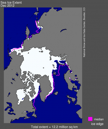
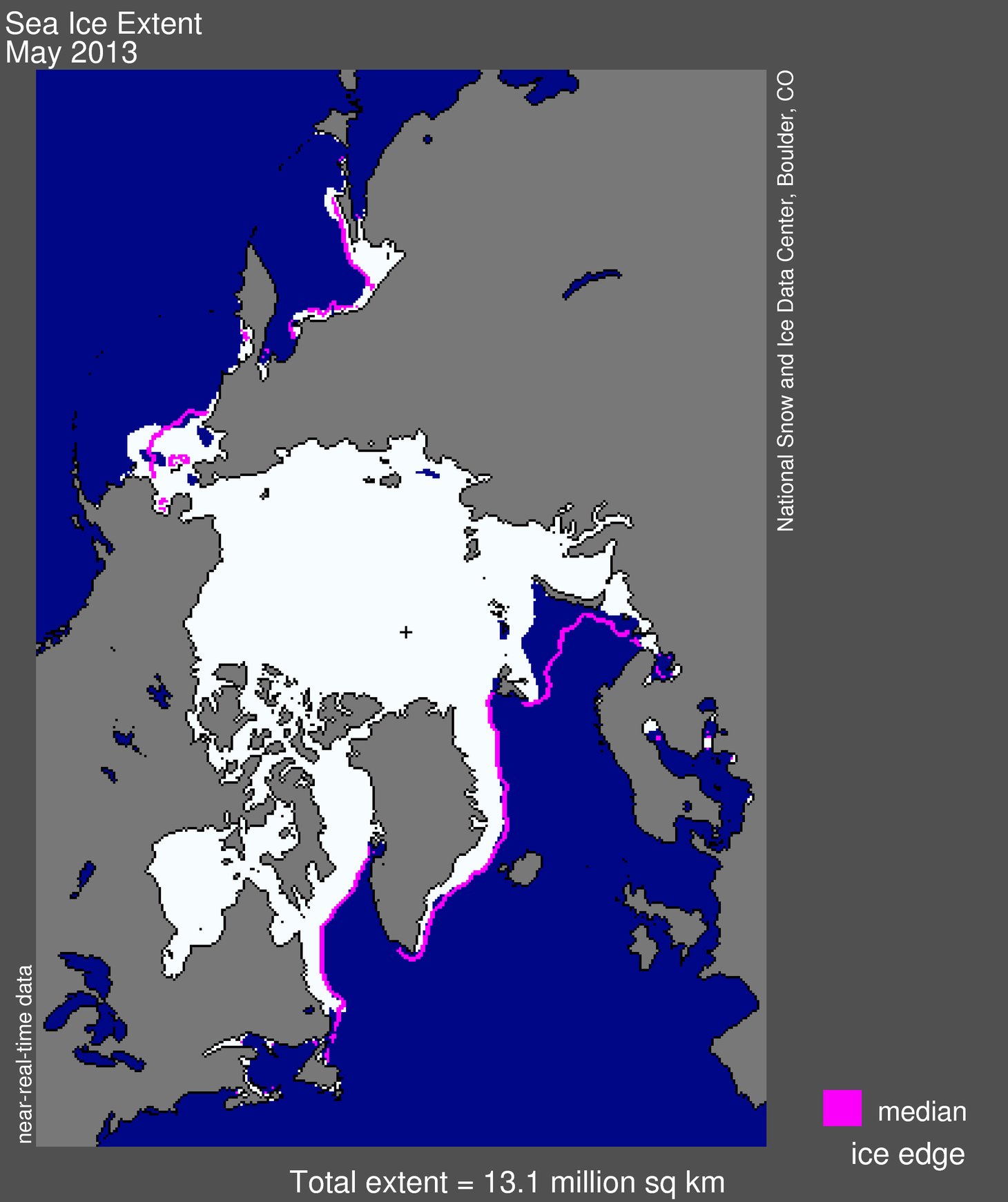
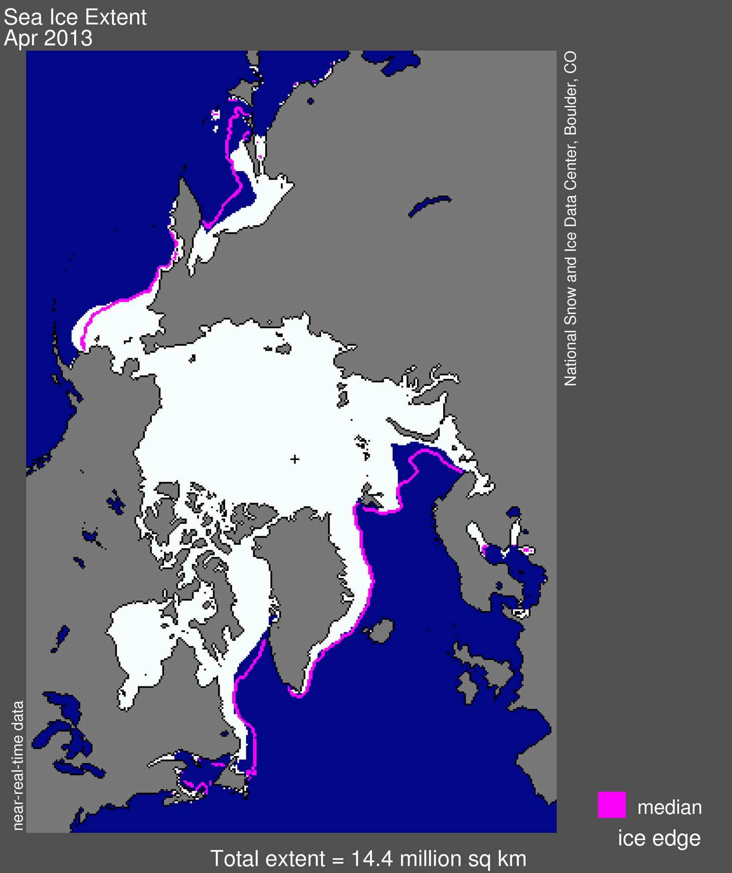
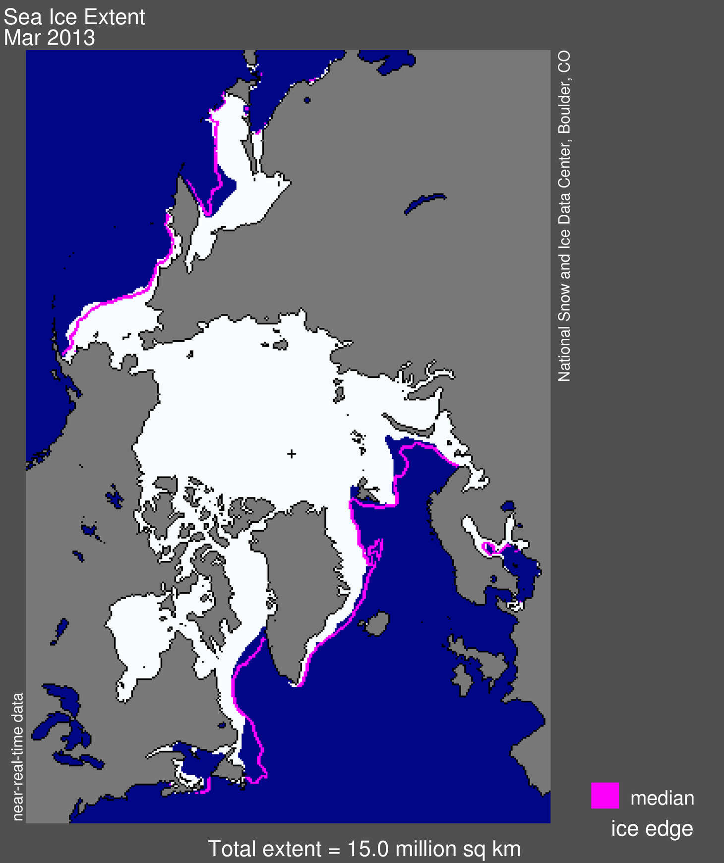
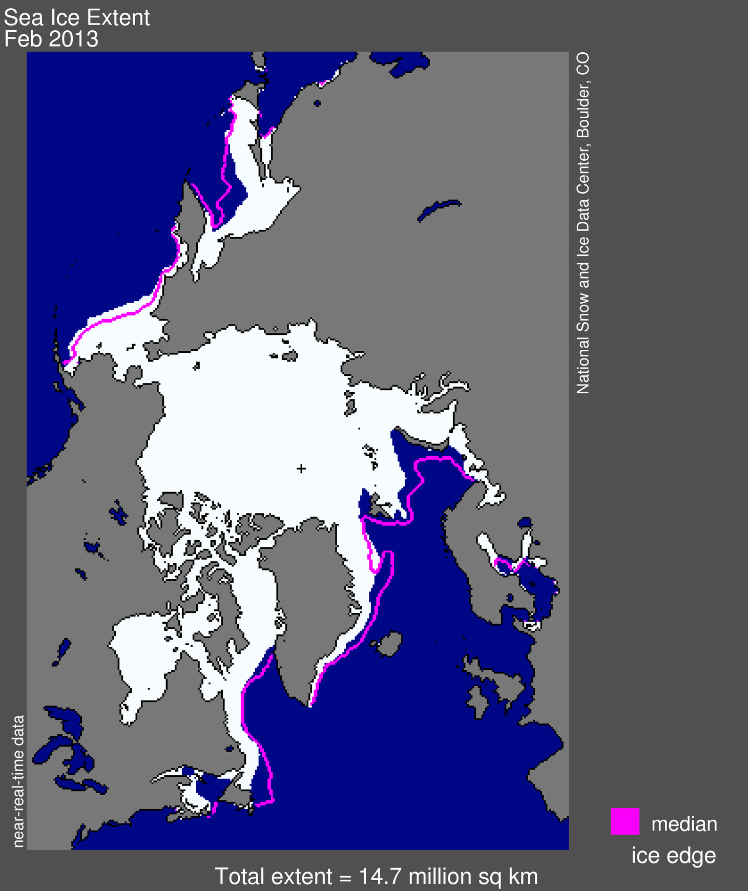
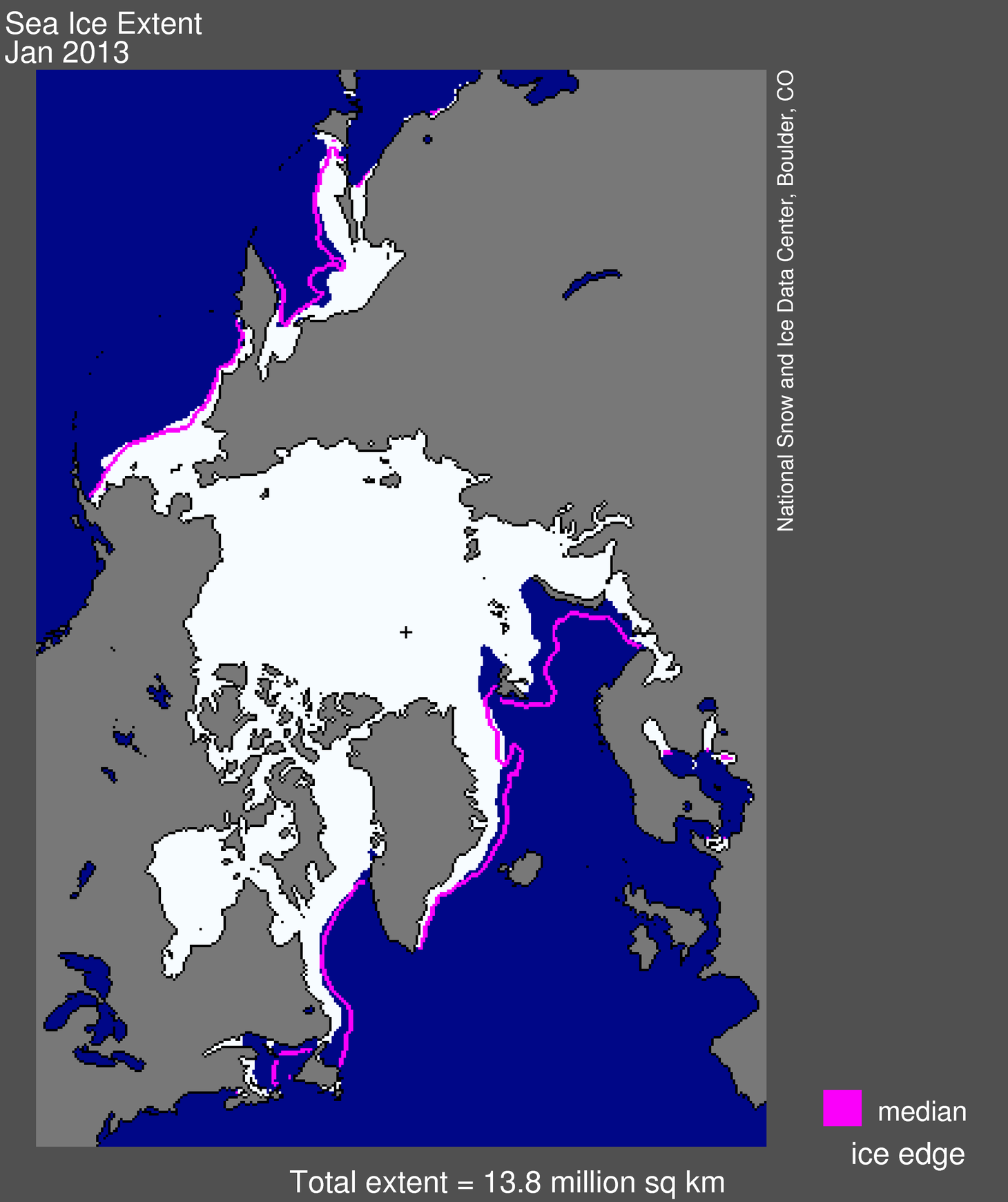
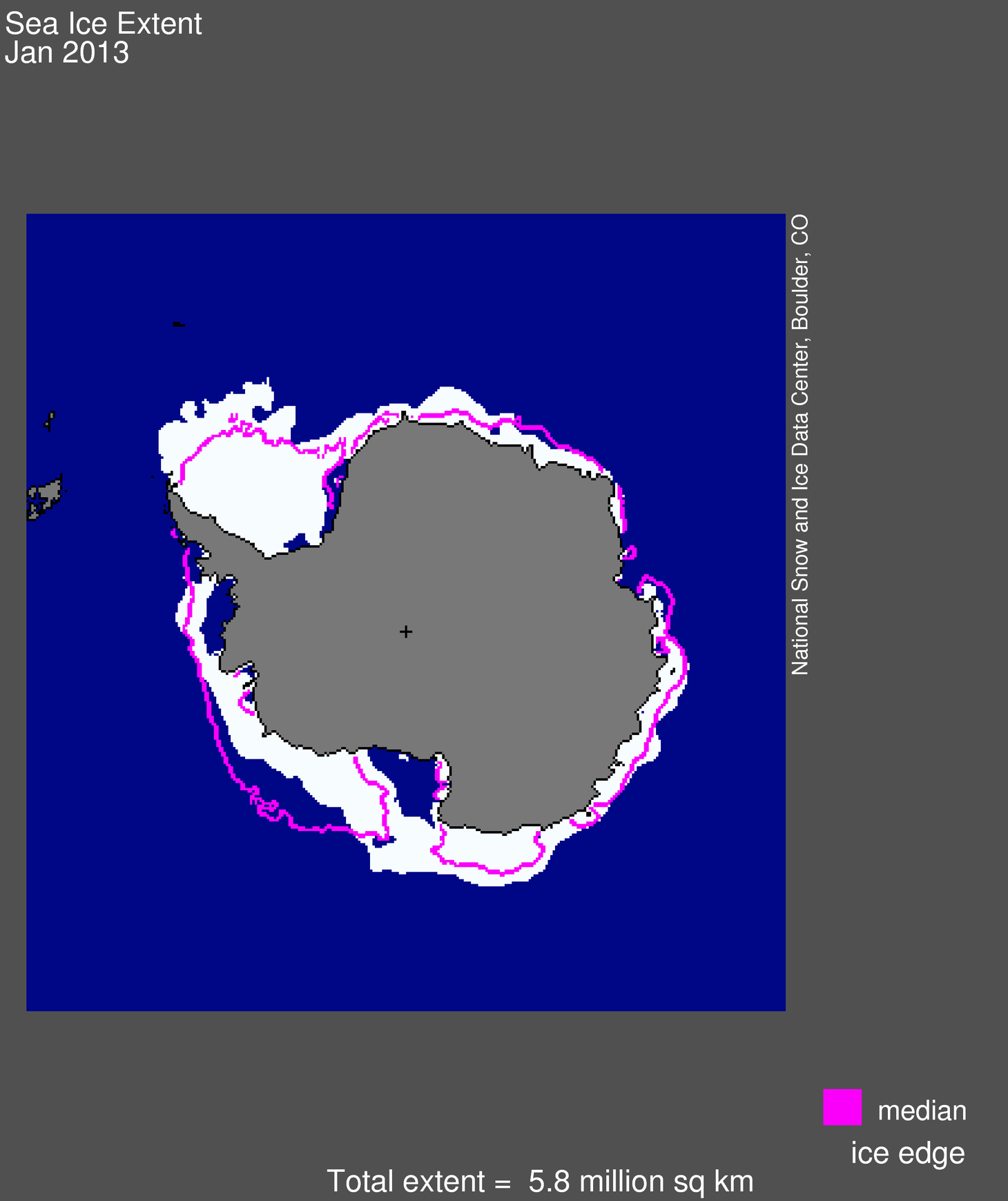
Figure 1. Arctic sea ice extent for December 2012 was 12.20 million square kilometers (4.71 million square miles). The magenta line shows the 1979 to 2000 median extent for that month. The black cross indicates the geographic North Pole. Sea Ice Index data. About the data

Credit: National Snow and Ice Data Center
High-resolution image

The average sea ice extent for December 2012 was 12.20 million square kilometers (4.71 million square miles). This is 1.16 million square kilometers (448,000 square miles) below the 1979 to 2000 average for the month, and is the second-lowest December extent in the satellite record.

At the end of December, ice extent in the Atlantic sector remained far below normal, as parts of the Kara and Barents seas remained ice-free. Ice has also been slow to form in the Labrador Sea, while Hudson Bay is now completely iced over. On the Pacific side, ice extent is slightly above normal, with the ice edge in the Bering Sea extending further to the south than usual. The Bering Sea has seen above-average winter ice extent in recent years and is the only region of the Arctic that has exhibited a slightly positive trend in ice extent during the winter months.

Conditions in context

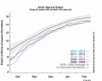
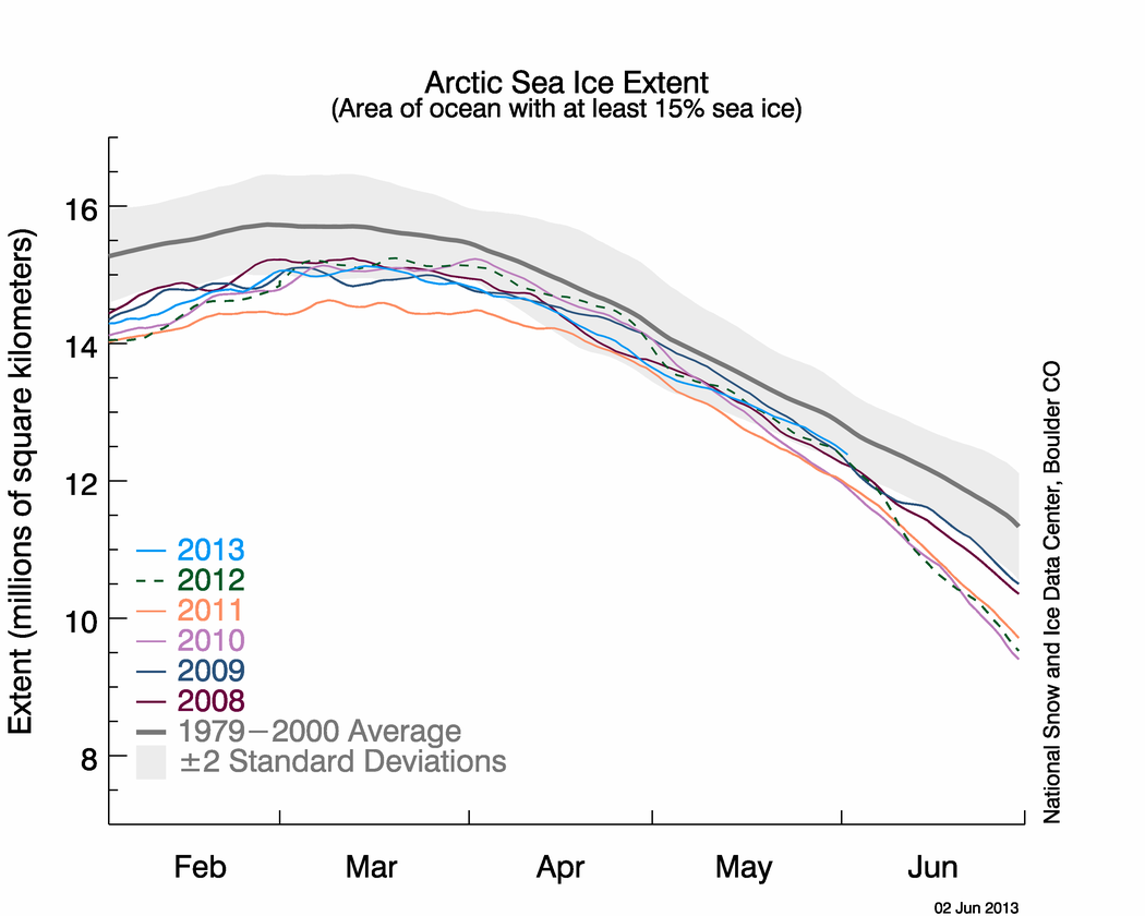
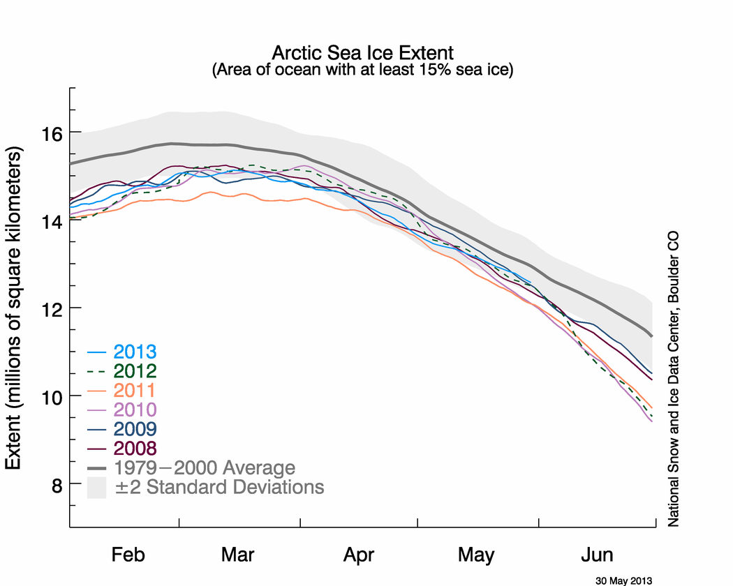
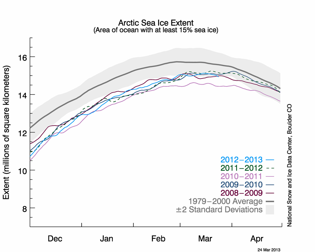
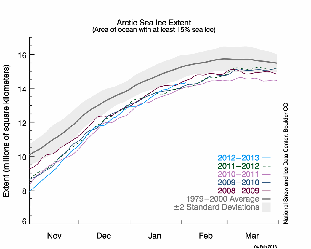
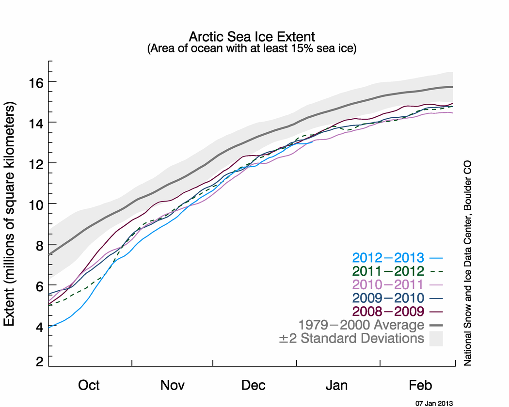
Figure 2. The graph above shows Arctic sea ice extent as of January 7, 2013, along with daily ice extent data for the previous five years. 2012 to 2013 is shown in blue, 2011 to 2012 in green, 2010 to 2011 in pink, 2009 to 2010 in navy, and 2008 to 2009 in purple. The 1979 to 2000 average is in dark gray. The gray area around this average line shows the two standard deviation range of the data. Sea Ice Index data.

Credit: National Snow and Ice Data Center
High-resolution image

Although the Arctic gained 2.33 million square kilometers of ice (900,000 square miles) through the month, ice extent in the region remained far below average. Ice growth remained slow in the Kara and Barents seas where air temperatures were 3 to 5 degrees Celsius (5 to 9 degrees Fahrenheit) higher than normal. Air temperatures over Greenland and the Canadian Archipelago were also slightly above average, while temperatures over Alaska were 2 to 7 degrees Celsius (4 to 13 degrees Fahrenheit) lower than average.

Winter sea ice variability is largely confined to the peripheral seas surrounding the Arctic Ocean. In the past, the dominant pattern of winter sea ice variability showed a distinct out-of-phase relationship between the Labrador and Greenland-Barents seas, with a less prominent seesaw pattern in the Pacific sector, between the Bering Sea and the Sea of Okhotsk. In recent winters however, this out-of-phase relationship no longer appears to hold in the Atlantic sector. Ice extent has remained below average in both the Labrador and the Barents seas.

Successive winters with anomalously low sea ice in the North Atlantic have led to higher mortality rates for seals in the region. The United States government recently added the bearded and ringed seals to the list of creatures threatened under the Endangered Species Act.

December 2012 compared to previous years

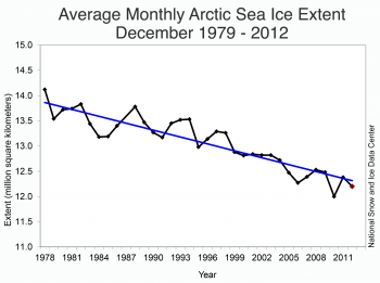
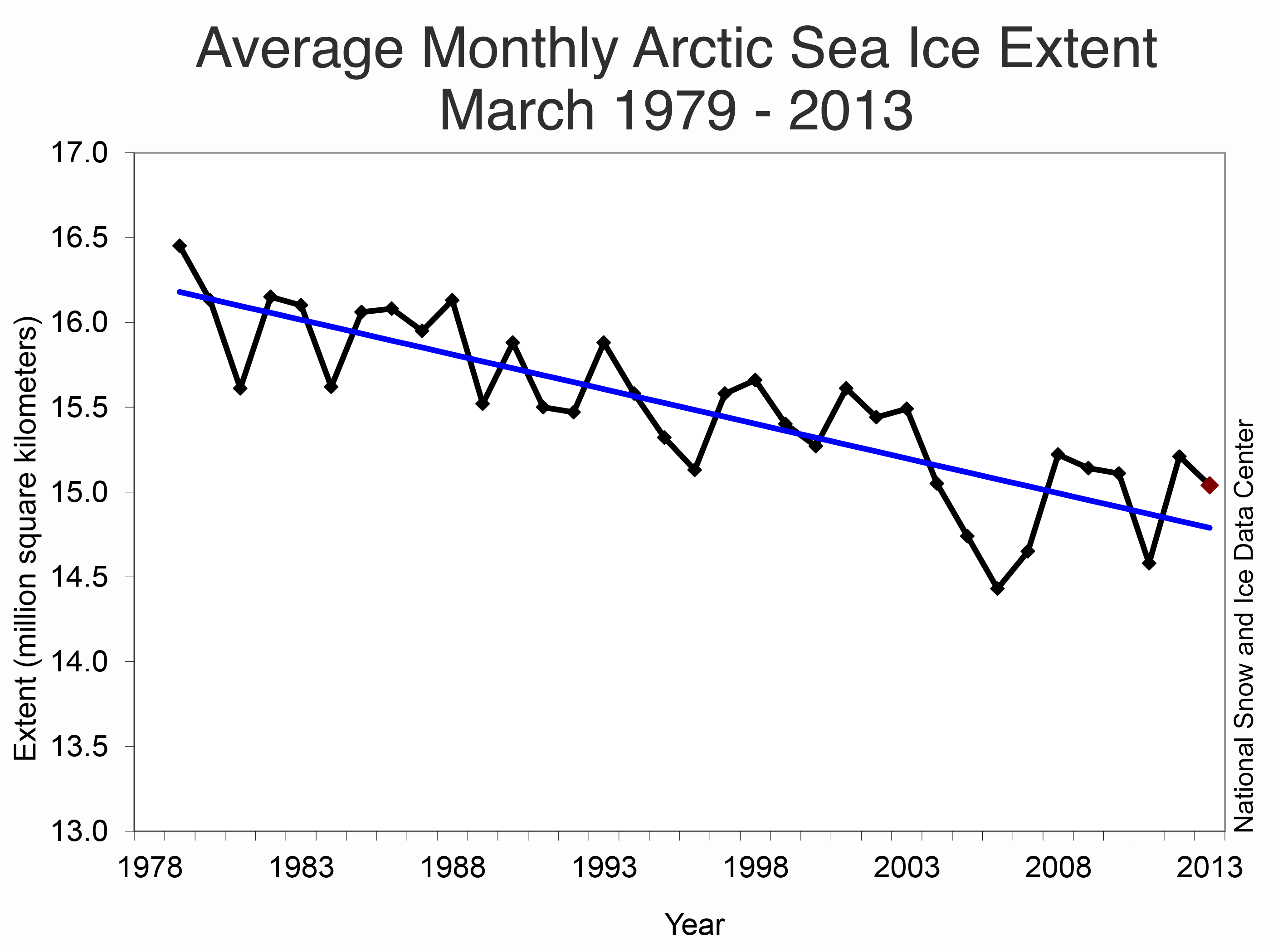
Figure 3. Monthly December ice extent for 1979 to 2012 shows a decline of -3.5(+/-0.6)% per decade.

Credit: National Snow and Ice Data Center
High-resolution image

Average Arctic sea ice extent for December 2012 was the second lowest for the month in the satellite record. Through 2012, the linear rate of decline for December ice extent is -3.5 percent per decade relative to the 1979 to 2000 average. While the winter ice extent for the Arctic as a whole shows only modest declines, large negative trends are now found in nearly all of the peripheral seas, with the exception of the Bering Sea.

Negative Arctic Oscillation

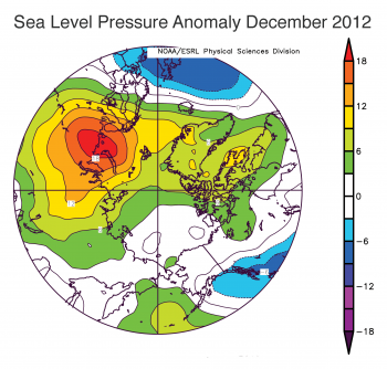
Figure 4. This image shows sea level pressure anomalies averaged for December 2012, compared to averages over the period 1981 to 2010. Sea level pressure was above average over Eurasia, extending into the Kara and Barents seas, and across Greenland and the Canadian Archipelago.

Credit: NSIDC courtesy NOAA/ESRL PSD
High-resolution image

The most important mode of variation in the Arctic’s winter atmospheric circulation is the Arctic Oscillation. When the Arctic Oscillation is in a negative mode or phase, sea level pressure is higher than normal over the central Arctic and lower than normal over middle latitudes. This pattern tends to keep the high Arctic relatively warm. It brings colder weather to Europe and North America because air masses can cross into and out of the high Arctic more easily. This pattern tends to favor the retention of thick ice in the Arctic basin by reducing the outflow of ice through the Fram Strait and strengthening the Beaufort Gyre, a clockwise circular pattern of ice drift in the central Arctic. The opposite conditions generally hold for a positive Arctic Oscillation pattern.

The specific influence of this winter’s negative Arctic Oscillation will depend not only on the strength of the sea level pressure anomaly, but also on the location of the sea level pressure center of action. While a negative Arctic Oscillation pattern tends to favor more ice in summer, this was not the case during the extreme negative Arctic Oscillation winter of 2009 to 2010.

The overall effect on the ice cover remains to be seen. Recent studies have argued that that strong warming of the atmosphere in autumn from summer sea ice loss favor the negative Arctic Oscillation phase.

2012 Year in Review

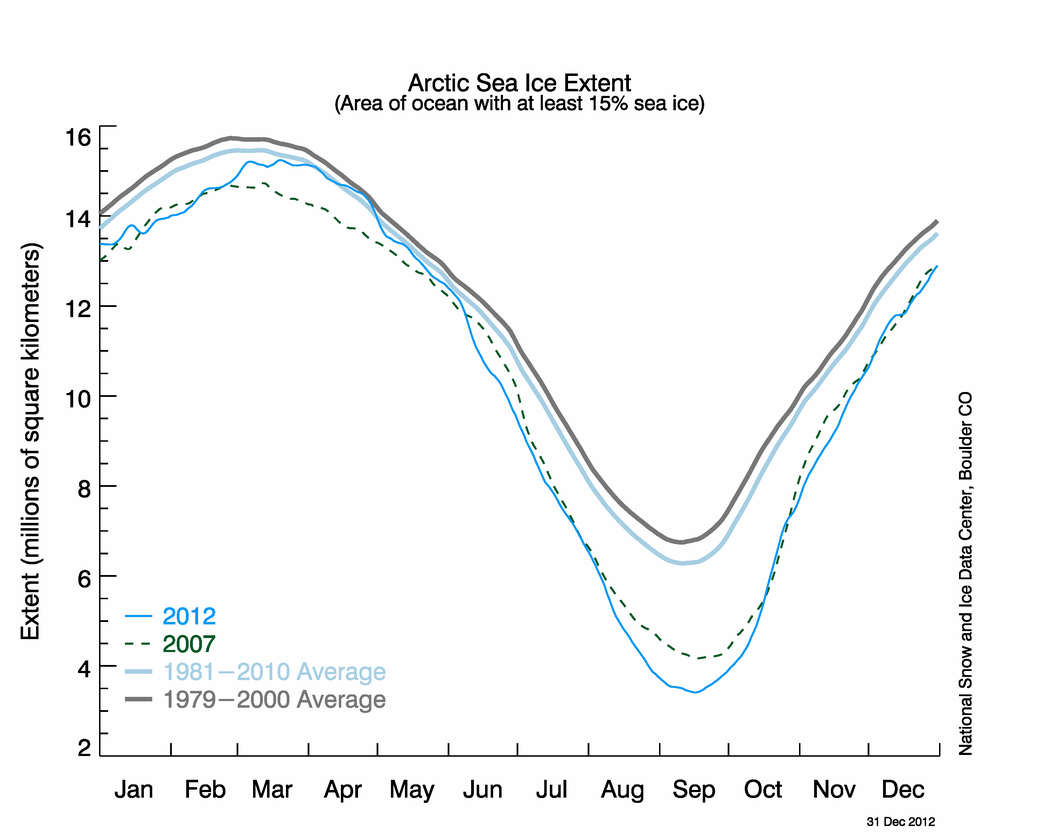
Figure 5. The graph above shows January to December Arctic sea ice extent for the two lowest extent years in the satellite record. Year 2012 is shown in blue and 2007 is shown in green. The 1981 to 2010 average is shown in light blue while the 1979 to 2000 average is in dark gray. Sea Ice Index data. About the data

Credit: National Snow and Ice Data Center
High-resolution image

While the year began with lower than average extent for the Arctic as a whole, extent in the Bering Sea was at record high levels for much of the winter. The seasonal decline of ice extent began slowly, such that in mid-April, extent for the Arctic as a whole was briefly near average levels.

Extent began dropping rapidly beginning in May, and by the end of the melt season on September 16, extent was at the lowest level recorded in the satellite record of 3.41 million square kilometers (1.32 million square miles). While summer weather conditions were not as favorable for ice loss as during 2007, the year of the previous record low, an unusually strong cyclone in August helped to quickly break up the already thin and fragmented ice cover in the Chukchi Sea. This cyclone—remarkable in its intensity and its duration—lasted for thirteen days, of which ten days were spent in the Arctic basin.

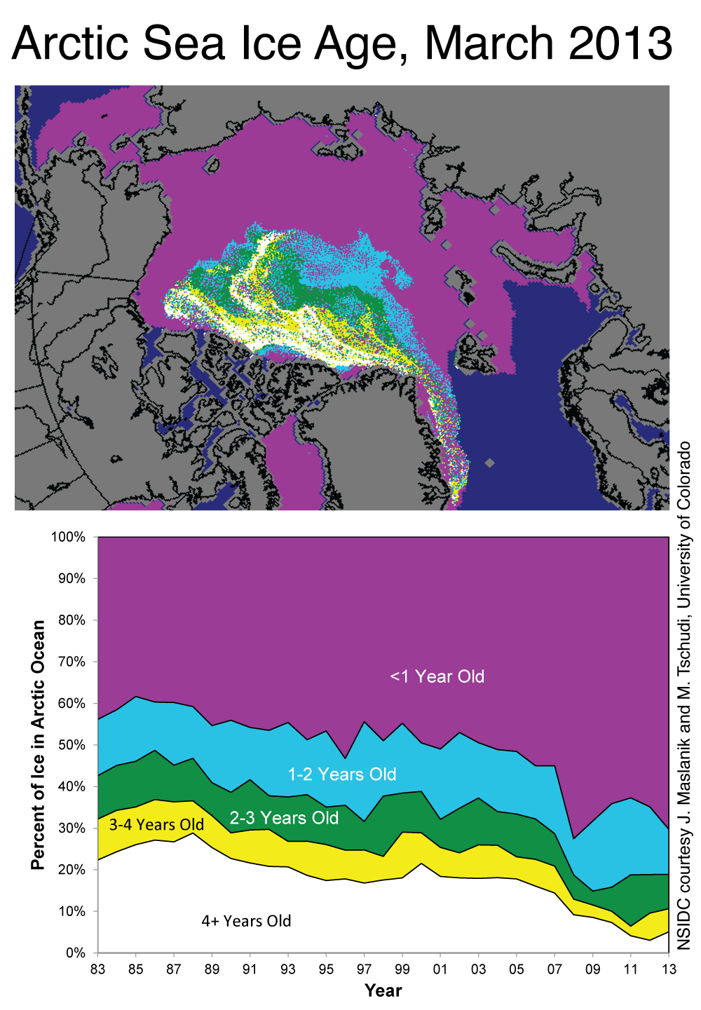
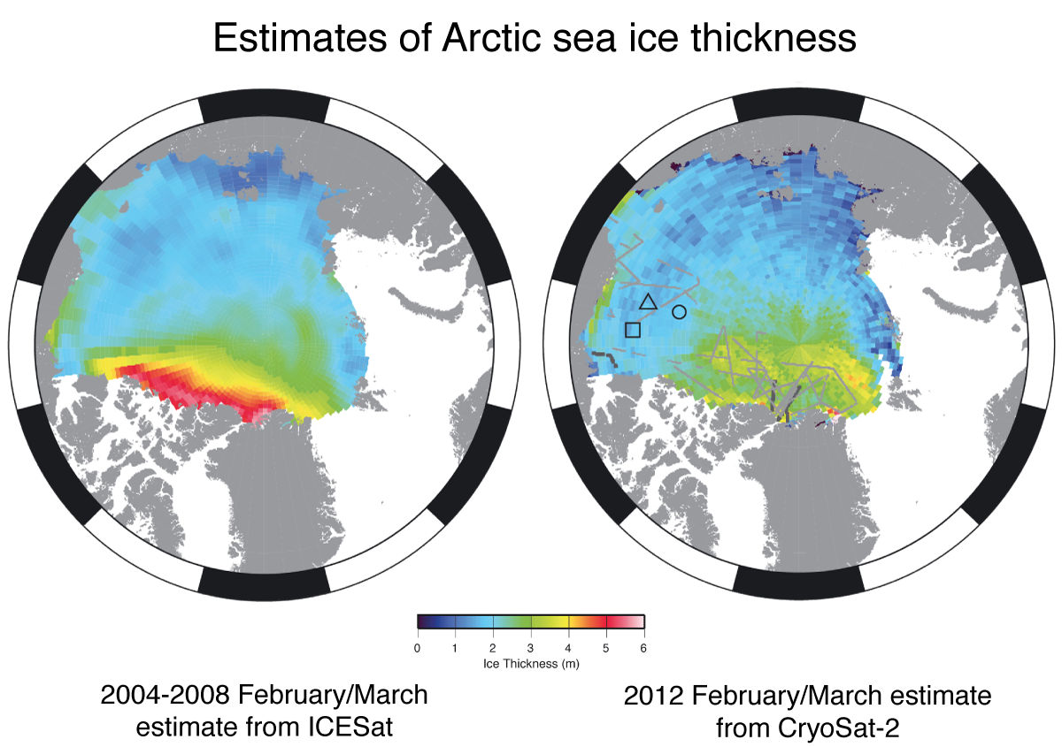
While it appears that a record low extent would have been reached even without the cyclone, thinning over the last several decades has made the ice more vulnerable to such storms, compared to earlier decades when the Arctic Ocean was dominated by thick, multiyear ice.

The annual average extent is now declining at a rate of -4.5 percent per decade relative to the 1979 to 2000 average and -4.6 percent per decade relative to the 1981 to 2010 average. The 1981 to 2010 period is the 30-year climatology used by the National Oceanic and Atmospheric Administration (NOAA) for their climate normals. Thirty years is a commonly-used period to define average or normal climate conditions. It is long enough to capture much climate variability, such as the different modes of the Arctic Oscillation, and short enough to be relevant for human timescales, such as agricultural cycles. NOAA updates its climate normals every ten years. For Arctic sea ice, use of the 1981 to 2010 period results in a lower extent than the 1979 to 2000 period, as seen in Figure 5, because the low extents of the last decade are included.

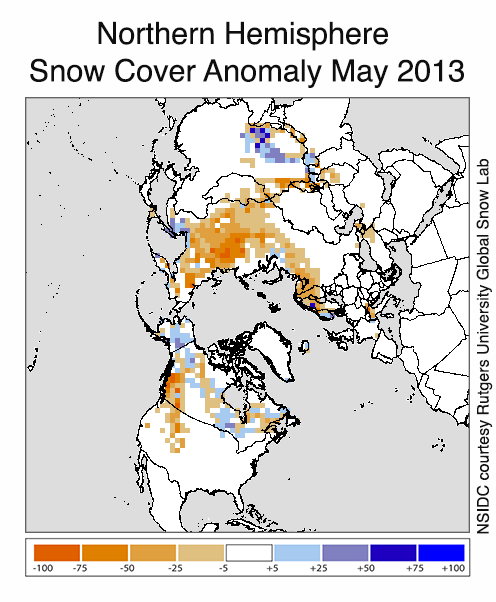
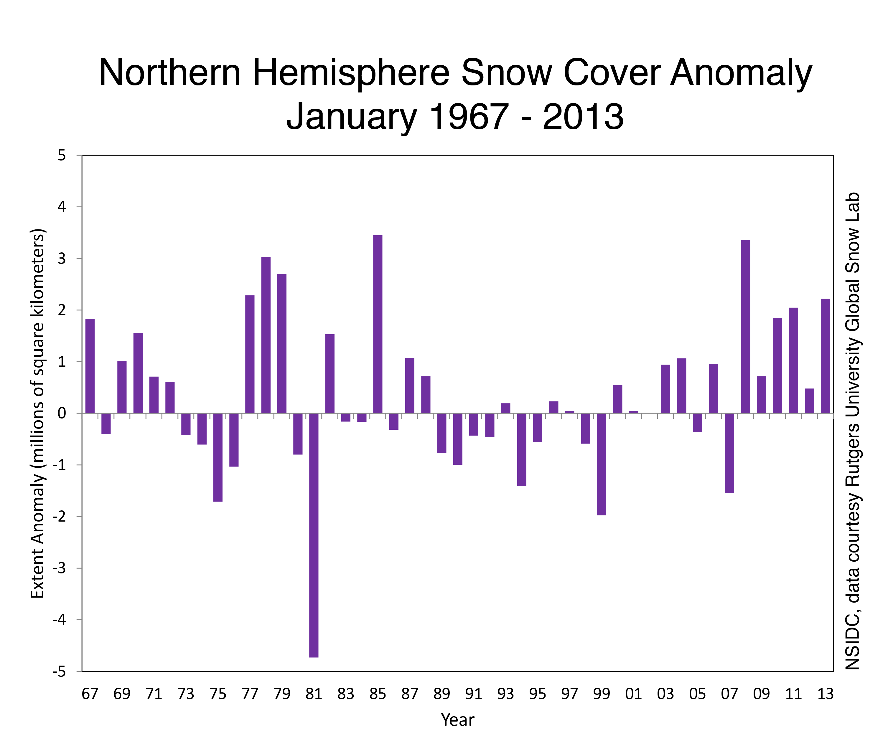
Record low ice extent was not the only remarkable event in the north. In June, Northern Hemisphere land snow cover set a new record for the least amount of snow cover in the 45-year record. A month later, the Greenland ice sheet experienced melt over more than 90 percent of its surface area, the largest melt extent recorded during the satellite data record.

Further reading

Simmonds, I. and I. Rudeva.  2012. The great Arctic cyclone of August 2012. Geophysical Research Letters 39, L23709, doi:10.1029/2012GL054259.

Jaiser, R., K. Dethloff, D. Handorf, A. Rinke, and J. Cohen. 2011. Impact of sea ice cover changes on the Northern Hemisphere atmospheric winter circulation. Tellus A, 64, 11595, doi:10.3402/tellusa.v64i0.11595.

Stroeve, J. C., J. Maslanik, M. C. Serreze, I. Rigor, W. Meier, and C. Fowler. 2011. Sea ice response to an extreme negative phase of the Arctic Oscillation during winter 2009/2010, Geophysical Research Letters 38, L02502, doi:10.1029/2010GL045662.