Sea ice declined at a near average rate through the first half of July as low sea level pressure dominated the Arctic Ocean. Wind patterns caused smoke from Siberian forest fires to sweep over the ice.

Overview of conditions

Figure 1. Arctic sea ice extent for July 15, 2018 was 8.5 million square kilometers (3.3 million square miles). The orange line shows the 1981 to 2010 average extent for that day. Sea Ice Index data. About the data

Credit: National Snow and Ice Data Center
High-resolution image

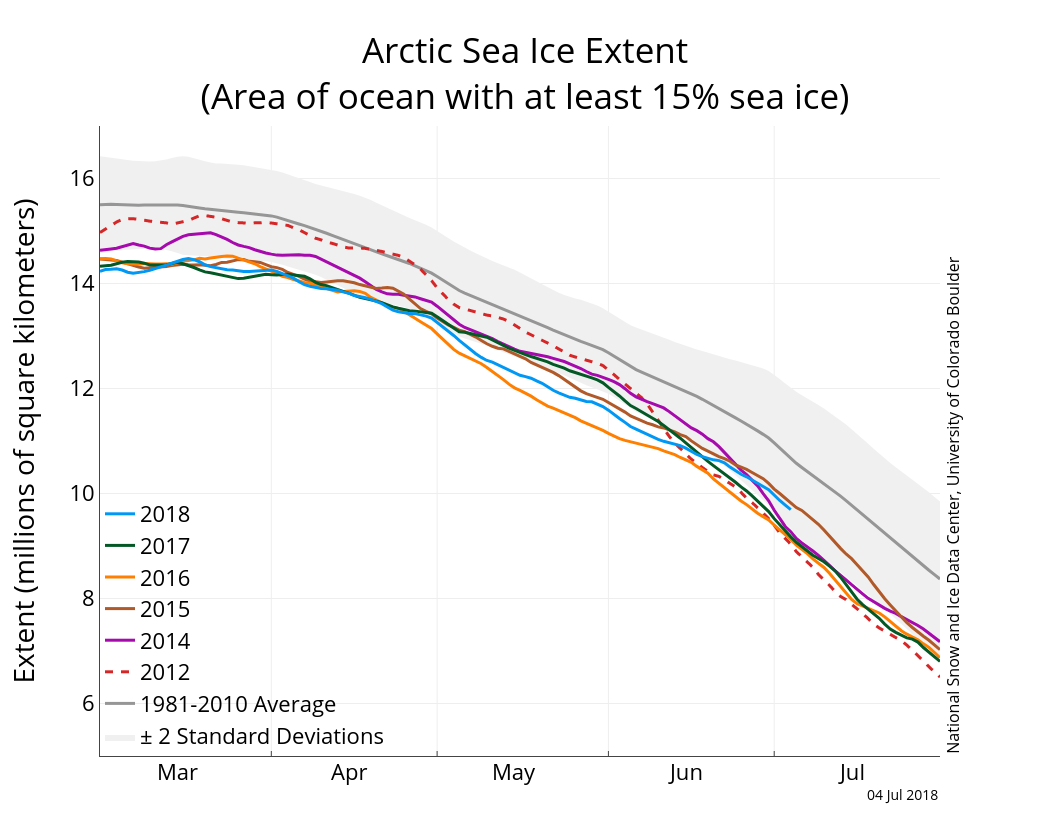
As of July 15, Arctic sea ice extent was 8.5 million square kilometers (3.3 million square miles). This is 1.24 million square kilometers (479,000 square miles) below the 1981 to 2010 average, but 670,000 square kilometers (259,000 square miles) above the record low for this day in 2011. While total Arctic sea ice extent was tracking at record low levels during winter, the rate of summer ice loss has been unremarkable thus far. Thus far in July, ice retreat has been most pronounced in the Kara Sea, whereas in the Beaufort Sea, the ice edge expanded slightly southwards. The ice edge has changed little within the Barents and East Greenland Seas on the Atlantic side, and retreat has been sluggish in the Chukchi Sea on the Pacific side of the Arctic Ocean.

Conditions in context

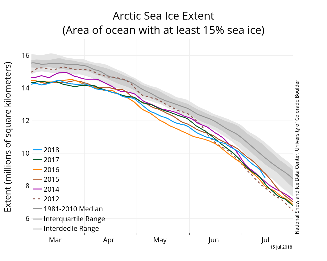
Figure 2a. The graph above shows Arctic sea ice extent as of July 15, 2018, along with daily ice extent data for four previous years and the record low year. 2018 is shown in blue, 2017 in green, 2016 in orange, 2015 in brown, 2014 in purple, and 2012 in dotted brown. The 1981 to 2010 median is in dark gray. The gray areas around the median line show the interquartile and interdecile ranges of the data. Sea Ice Index data.

Credit: National Snow and Ice Data Center
High-resolution image

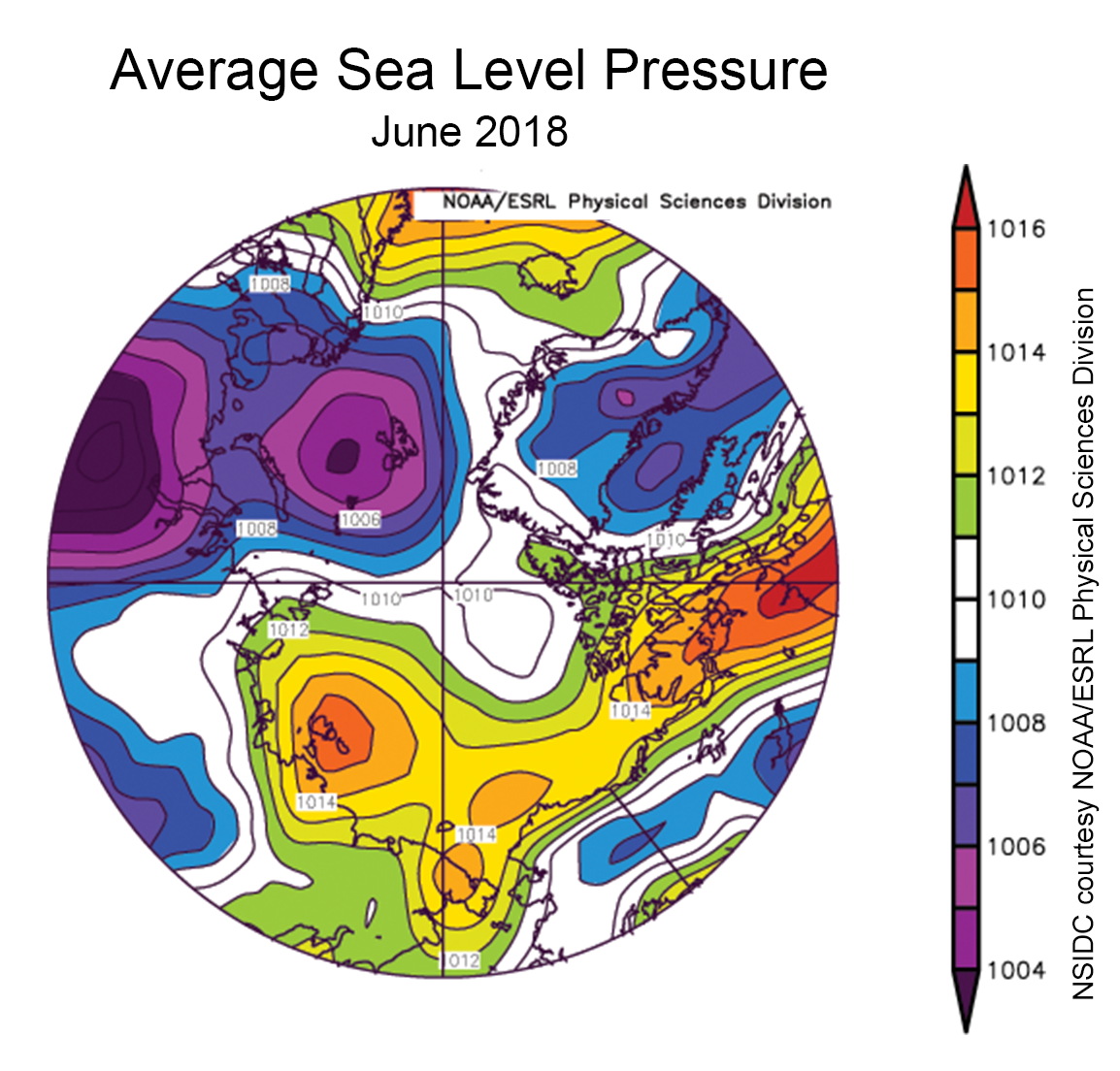
Figure 2b. This plot shows average sea level pressure in the Arctic, in millibars, for July 1 to 15, 2018. Yellows and reds indicate higher than average sea level pressure; blues and purples indicate lower than average sea level pressure.

Credit: NSIDC courtesy NOAA Earth System Research Laboratory Physical Sciences Division
High-resolution image

Through the first two weeks of July, ice extent declined at a rate of 134,000 square kilometers (52,000 square miles) per day, which is near the 1981 to 2010 average. The spatial pattern of ice loss has not changed much since the end of June, with minimal ice loss around the entire ice edge. The Beaufort Sea saw some increase in extent due to the transport of ice from the north. Low sea level pressure dominated the central Arctic Ocean and Greenland. Typically, this pattern, associated with counterclockwise (cyclonic) winds is associated with cool conditions and also causes ice divergence, helping to spread the ice cover over a larger area. However, air temperatures over the pole and the East Siberian and Chukchi Seas at the 925 hPa level (approximately 2,500 feet above the surface) ranged 1 to 2 degrees Celsius (2 to 4 degrees Fahrenheit) above average for the first part of July. Regions with below average air temperatures were found in the Kara, Laptev, and Beaufort Seas (-1 to -3 degrees Celsius or -2 to -5 degrees Fahrenheit below average).

The passive microwave data show a decrease in ice concentration in several areas of the Arctic Ocean, particularly in northern areas of the Beaufort and Chukchi Seas. This is not necessarily a real decrease—it manifests as surface melt and the development of melt ponds on the ice surface. Microwave emission is sensitive to the freeze-thaw state of water. Liquid water atop the ice surface changes the returned signal, mimicking a reduced sea ice concentration. Because the calculation of ice extent does not consider concentration (except for the 15 percent concentration threshold), extent values are much less sensitive to this melt effect. During the melt season, ice extent provides a more consistent and reliable measure of total ice cover.

Siberian smoke over the Arctic Ocean

Figure 3. These images from the NASA Moderate Resolution Imaging Spectroradiometer (MODIS) sensor show the Arctic Ocean and surrounding land from July 3 to 6, 2018. Blue arrows indicate smoke that had drifted from fires in Siberia.

Credit: NASA
High-resolution image

Fires in the western United States have been much in the news lately. Less noted are significant fires in Siberia. Over several days at the beginning of July, smoke from these fires was brought into the Arctic Ocean by winds associated with the pattern of low pressure in the region. The smoke streamed over the East Siberian, Chukchi, and Beaufort Seas and eventually across Alaska into northern Canada.

The smoke has two potential effects on sea ice. First, as it drifts over the ice, the smoke particles scatter solar radiation and reduce how much is received at the surface. This has a cooling effect that will tend to reduce the rate of ice loss. However, smoke particles that settle onto the ice will darken the surface, thus decreasing the reflectivity of the surface, or albedo. This increases the amount of solar energy absorbed by the ice and enhances melt. The atmospheric scattering effect of the smoke is short term and dissipates after the smoke drifts away. The surface albedo effect has a longer-term impact and could serve to enhance melt rates through the summer. The magnitude of the effect will depend on how many smoke particles are deposited on the surface, the albedo of the surface that the particles fall on, and the amount of cloud cover which reduces the incoming sunlight. The biggest effect would be on bright, snow-covered ice. It would be smaller on darker melting ice and melt ponds, and there would be no effect in open water areas.

Arctic sea ice extent declined at a slightly slower-than average pace in June. Despite the slow loss, warm conditions and winds from the south developed a large area of open water in the Laptev Sea.

Overview of conditions

Figure 1. Arctic sea ice extent for June 2018 was 10.7 million square kilometers (4.1 million square miles). The magenta line shows the 1981 to 2010 average extent for that month. Sea Ice Index data. About the data

Credit: National Snow and Ice Data Center
High-resolution image

Arctic sea ice extent for June 2018 averaged 10.7 million square kilometers (4.1 million square miles). This was 1.05 million square kilometers (405,000 square miles) below the 1981 to 2010 average and 360,000 square kilometers (139,000 square miles) above the record low June extent set in 2016. This was the fourth lowest June average extent in the satellite record.

Extent at the end of June remained below average in the Chukchi Sea, but because of slow retreat through June in the region, extent in the Chukchi is now closer to average than was the case at the end of May. The Barents Sea and East Siberian Sea also have extents well below average at the end of June. Most of the ice in the Sea of Okhotsk has melted. Ice has been retreating in the west side of Hudson Bay where extent is below average. However, this is countered by above average extent in the eastern side of the bay. Notably, a large area of open water has developed in the Laptev Sea, leading to record low extents in that region during the first half of June.

Conditions in context

Figure 2. The graph above shows Arctic sea ice extent as of July, 4, 2018, along with daily ice extent data for four previous years and 2012, the year with record low minimum extent. 2018 is shown in blue, 2017 in green, 2016 in orange, 2015 in brown, 2014 in purple, and 2012 in dotted brown. The 1981 to 2010 median is in dark gray. The gray areas around the median line show the interquartile and interdecile ranges of the data. Sea Ice Index data.

Credit: National Snow and Ice Data Center
High-resolution image

Figure 3a. This plot shows the average sea level pressure in the Arctic at the 925 hPa level, in millibars, for June 2018. Yellows and reds indicate higher than average air pressure; blues and purples indicate lower than average air pressure.

Credit: NSIDC courtesy NOAA Earth System Research Laboratory Physical Sciences Division
High-resolution image

Figure 3b. This plot shows departure from average air temperature in the Arctic at the 925 hPa level, in degrees Celsius, for June 2018. Yellows and reds indicate higher than average temperature; blues and purples indicate lower than average temperature.

Credit: NSIDC courtesy NOAA Earth System Research Laboratory Physical Sciences Division
High-resolution image

The salient features of the atmospheric pattern for June include a region of low sea level pressure centered over the northern Barents Sea, and a high pressure cell centered over the Laptev Sea. A ridge of high pressure also extends eastward into northern Canada (Figure 3a). Winds from the south between the low pressure area in the Barents Sea and the high pressure area in the Laptev Sea gave rise to a pronounced region of above-average temperatures centered over Central Siberia and extending over the Laptev and East Siberian Seas (Figure 3b). However, elsewhere over the Arctic Ocean, temperatures were near average or slightly below average.

The temperature pattern is consistent with the early development of open water in the Laptev Sea. Extents in this area oscillated between slightly above and below the record low extent set in June 2014. Parts of the Laptev Sea opened as early as mid-April, likely due to winds transporting ice away from the fast ice zone (ice that is locked to the shoreline). While new ice formed in these open water areas, this ice was thin and prone to melting out once the summer melt season started.

Also of note was the passage of a strong cyclone in early June. This system moved into the Kara Sea on June 6, and reached a minimum central pressure of less than 970 hPa on June 7. By June 10, it had migrated into the Beaufort Sea. It dissipated on June 13.

June 2018 compared to previous years

Figure 4. Monthly June ice extent for 1979 to 2018 shows a decline of 4.1 percent per decade.

Credit: National Snow and Ice Data Center
High-resolution image

The linear rate of decline for June sea ice extent is 48,000 square kilometers (18,500 square miles) per year, or 4.1 percent per decade relative to the 1981 to 2010 average. Ice loss during the month was 1.6 million square kilometers (618,000 square miles), somewhat slower than the 1981 to 2010 average loss of 1.7 million square kilometers (656,000 square miles) for the month. Clearly the early ice losses in the Laptev Sea, associated with warm conditions over the region, could not make up for slower retreats elsewhere.

New insights into warming in the northern Barents Sea

An interesting feature of recent years is a region of unusually high winter air temperatures, or a winter hotspot, over the northern Barents Sea. Previous studies have provided evidence linking the hotspot to a halocline retreat, which is a retreat or weakening of the cold, fresh waters at the ocean surface that prevent ocean heat imported from the Atlantic from mixing upwards. A new paper by Lind et al. (2018) argues that the hotspot is driven by the lack of sea ice transport. Sea ice is mostly fresh water (low salinity) and less is being transported into that region. Hence the ocean surface becomes less fresh over the northern Barents Sea, allowing the warm Atlantic water to mix upwards.

Antarctica in June

Figure 5. This plot shows departure from average air temperature in Antarctica at the 925 hPa level, in degrees Celsius, for June 2018. Yellows and reds indicate higher than average temperature; blues and purples indicate lower than average temperature.

Credit: NSIDC courtesy NOAA Earth System Research Laboratory Physical Sciences Division
High-resolution image

Sea ice expanded at a faster-than-average pace in June in the Southern Hemisphere, bringing Antarctic sea ice extent closer to typical ice extents for this time of year. This follows on the heels of a period of below-average ice extent since austral winter in 2016. Sea ice extent is near average in all sectors except the northeastern Weddell Sea, and a small area in the northern Davis Sea. Higher-than-average air temperatures prevailed in these regions, and cool conditions prevailed over the northern Ross Sea.

Antarctica’s sea ice and ice shelf disintegration

A new study in the Journal Nature found that reduced sea ice in the northwestern Weddell Sea and southern Bellingshausen Sea likely contributed to the weakening of major ice shelves prior to their disintegration in the 1990s and early 2000s. Loss of the sea ice buffer near Antarctica’s coast allows long-period ocean swell to flex ice shelves. Under ordinary conditions, this flexing has little effect. However, if the ice shelves have been pre-conditioned by seasonal melt-water flooding, the flexing by wave action in late summer can have a devastating effect. Minor flexure of the ice shelf plate allows water to infiltrate existing cracks and initiate fracturing of the ice.

Four major ice shelf break-up events in 1995 (Larsen A), 2002 (Larsen B), and 2008 and 2009 (Wilkins) all occurred after multiple weeks where no sea ice was present near the ice shelf fronts to dampen ocean swell. In the case of the Larsen A and B events, the loss of the ice shelves initiated a significant acceleration of the tributary glaciers. The study demonstrates that sea ice—a component of the cryosphere that is very sensitive to changing climate and ocean—has an important protective effect on the Antarctic ice sheet.

Further Reading

Lind, S., R. B. Ingvaldsen, and T. Furevik. 2018. Arctic warming hotspot in the Northern Barents Sea linked to declining sea-ice import. Nature Climate Change, doi:10.1038/s41558-018-0205-y.

Massom, R., T. A. Scambos, L. G. Benetts, P. Reid, V. A. Squire, and S. Stammerjohn. 2018. Antarctic ice shelf disintegration triggered by sea ice loss and ocean swell. Nature, 558, 383-389, doi:10.1038/s41586-018-0212-1.