As winter turns to spring, the seasonal decline in Arctic sea ice kicks into gear. April was marked by rapid ice loss at the beginning and end of the month. Air temperatures were higher than average over much of the Arctic Ocean. In the Antarctic, sea ice extent was the highest seen in April in the satellite record. This month we introduce data sets and online tools from new sensors that—combined with older sources—provide a more complete picture of ice thickness changes across the Arctic.

Overview of conditions

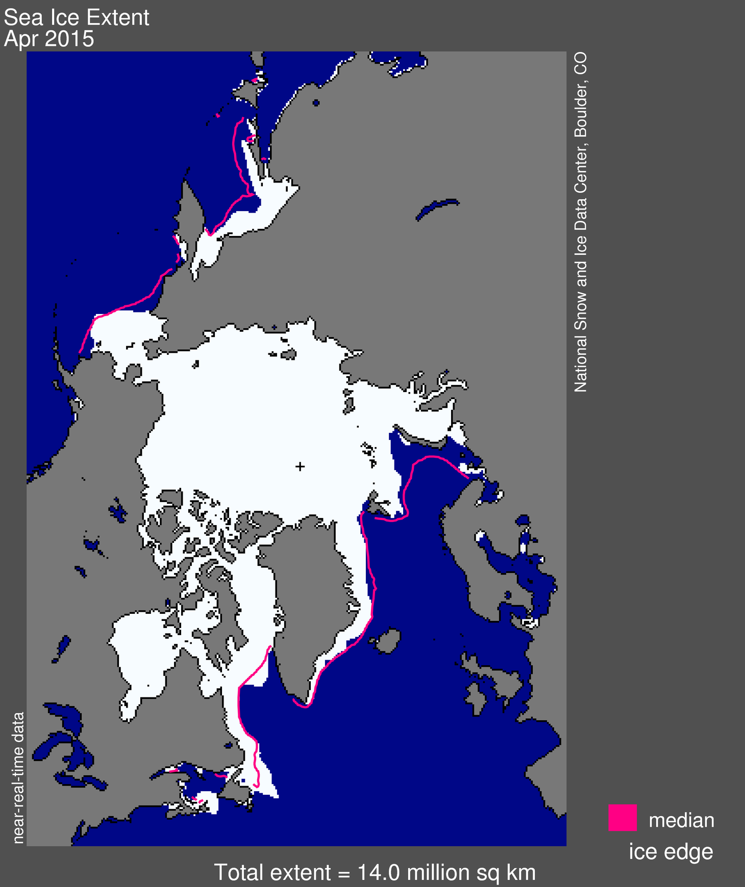
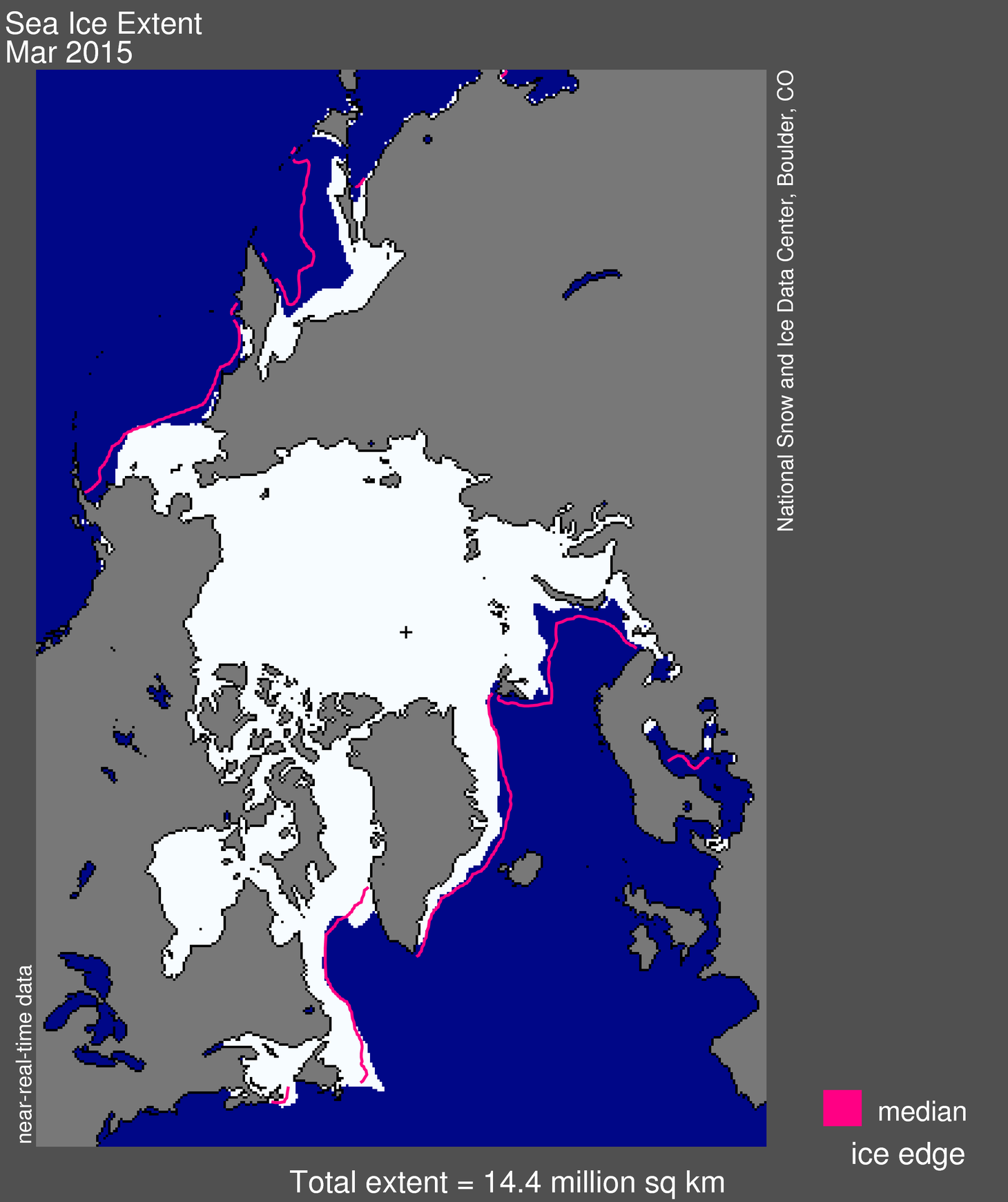
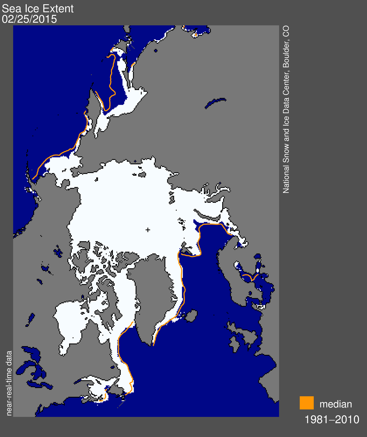
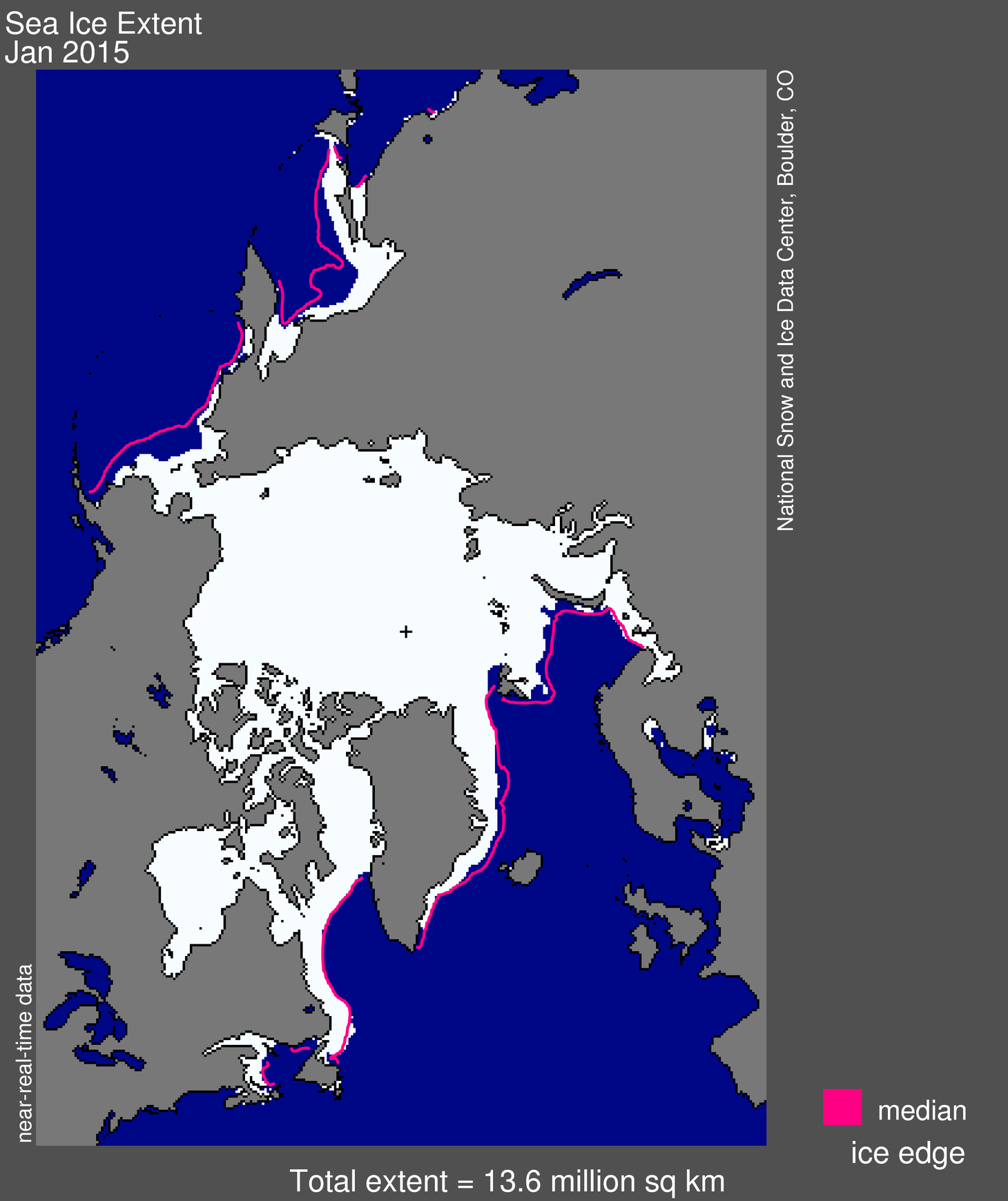
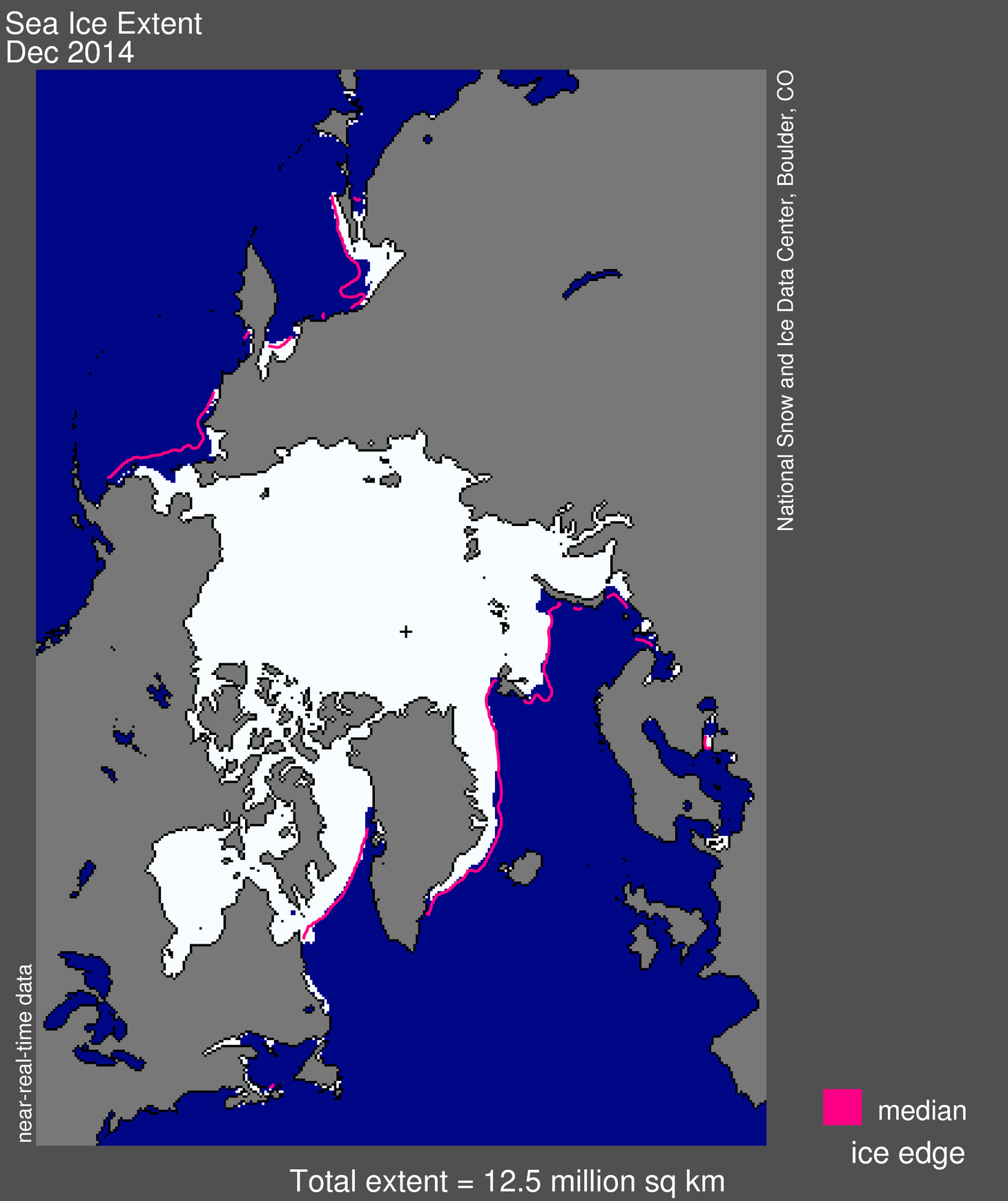
Figure 1. Arctic sea ice extent for April 2015 was 14.0 million square kilometers (5.4 million square miles). The magenta line shows the 1981 to 2010 median extent for that month. The black cross indicates the geographic North Pole. Sea Ice Index data. About the data

Credit: National Snow and Ice Data Center
High-resolution image

Arctic sea ice extent for April 2015 averaged 14.0 million square kilometers (5.4 million square miles), the second lowest April ice extent in the satellite record. It is 810,000 square kilometers (313,000 square miles) below the 1981 to 2010 long-term average of 15.0 million square kilometers (6.0 million square miles) and 80,000 square kilometers (31,000 square miles) above the previous record low for the month observed in 2007.

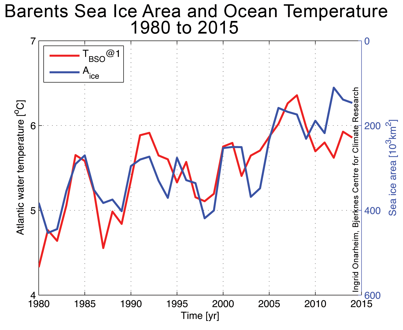
Ice extent remained below average in the Barents Sea, the Sea of Okhotsk, and the Bering Sea. Sea ice was slightly more extensive than average off Newfoundland, in the Davis Strait, and in the Labrador Sea. The Labrador Sea is an important breeding area for harp and hooded seals in early spring. More extensive ice in this region favors more seal cubs being fully weaned before the ice breaks up, increasing their chance of survival.

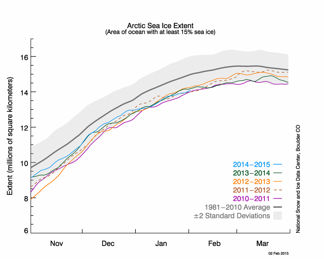
Conditions in context

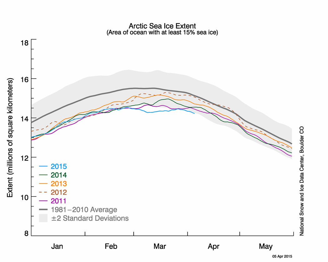
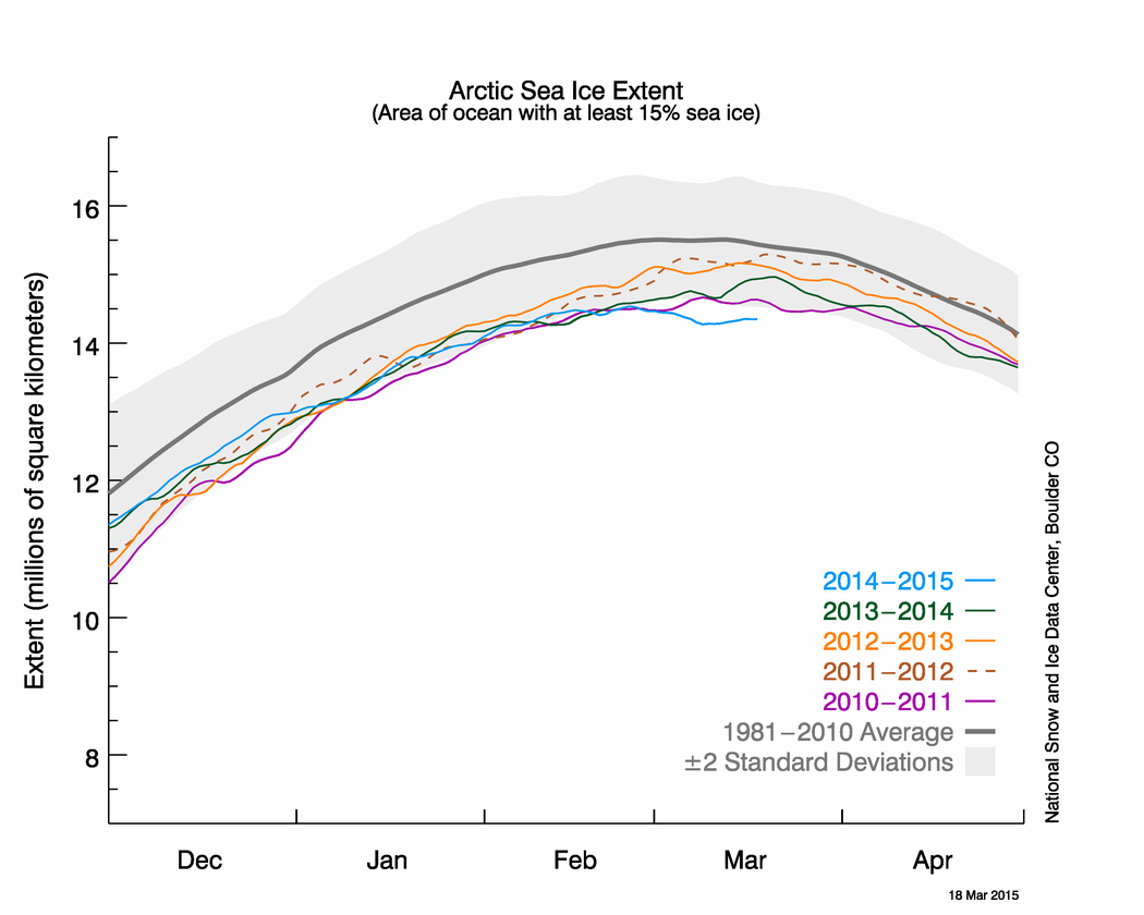
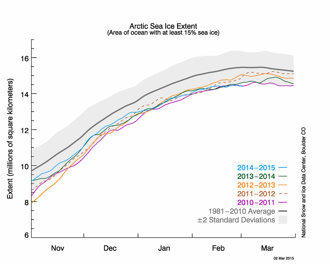
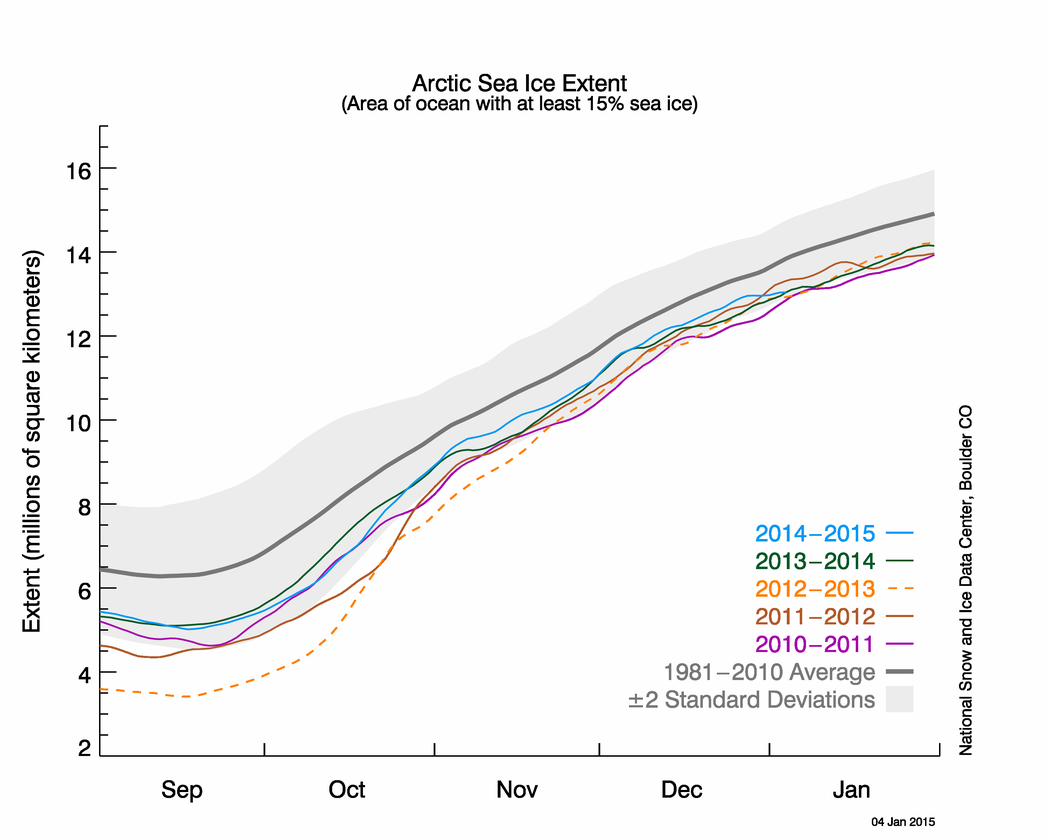
Figure 2. The graph above shows Arctic sea ice extent as of May 5, 2015, along with daily ice extent data for four previous years. 2015 is shown in blue, 2014 in green, 2013 in orange, 2012 in brown, and 2011 in purple. The 1981 to 2010 average is in dark gray. The gray area around the average line shows the two standard deviation range of the data. Sea Ice Index data.

Credit: National Snow and Ice Data Center
High-resolution image

During April, the decline in ice extent starts to accelerate, though the total ice loss over the month is generally small. April 2015 was marked by a fairly rapid decline during the first week of the month, little change during the middle of the month, and then a steep decline over the final week. Overall, extent decreased 862,000 square kilometers (333,000 square miles).

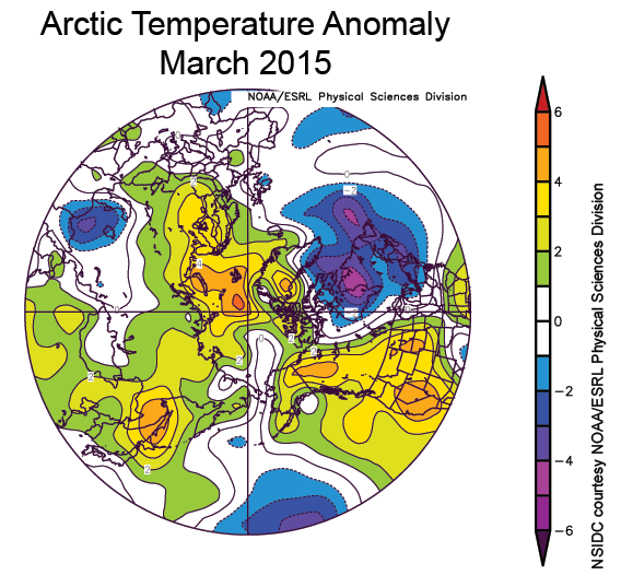
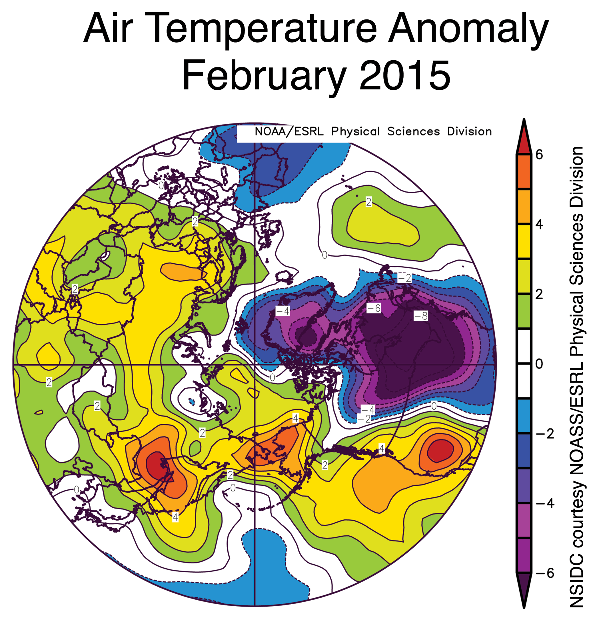
April was marked by higher than average 925 hPa air temperatures (1 to 3 degrees Celsius or 2 to 5 degrees Fahrenheit) throughout the Arctic, except for Greenland and the Canadian Archipelago where temperatures were 1 to 3 degrees Celsius (2 to 5 degrees Fahrenheit) below average. Temperatures were 6 to 8 degrees Celsius (11 to 14 degrees Fahrenheit) higher than average in the Kara Sea, linked to unusually low sea level pressure over the North Atlantic. Associated wind patterns also resulted in strong warming over the Eurasian Arctic.

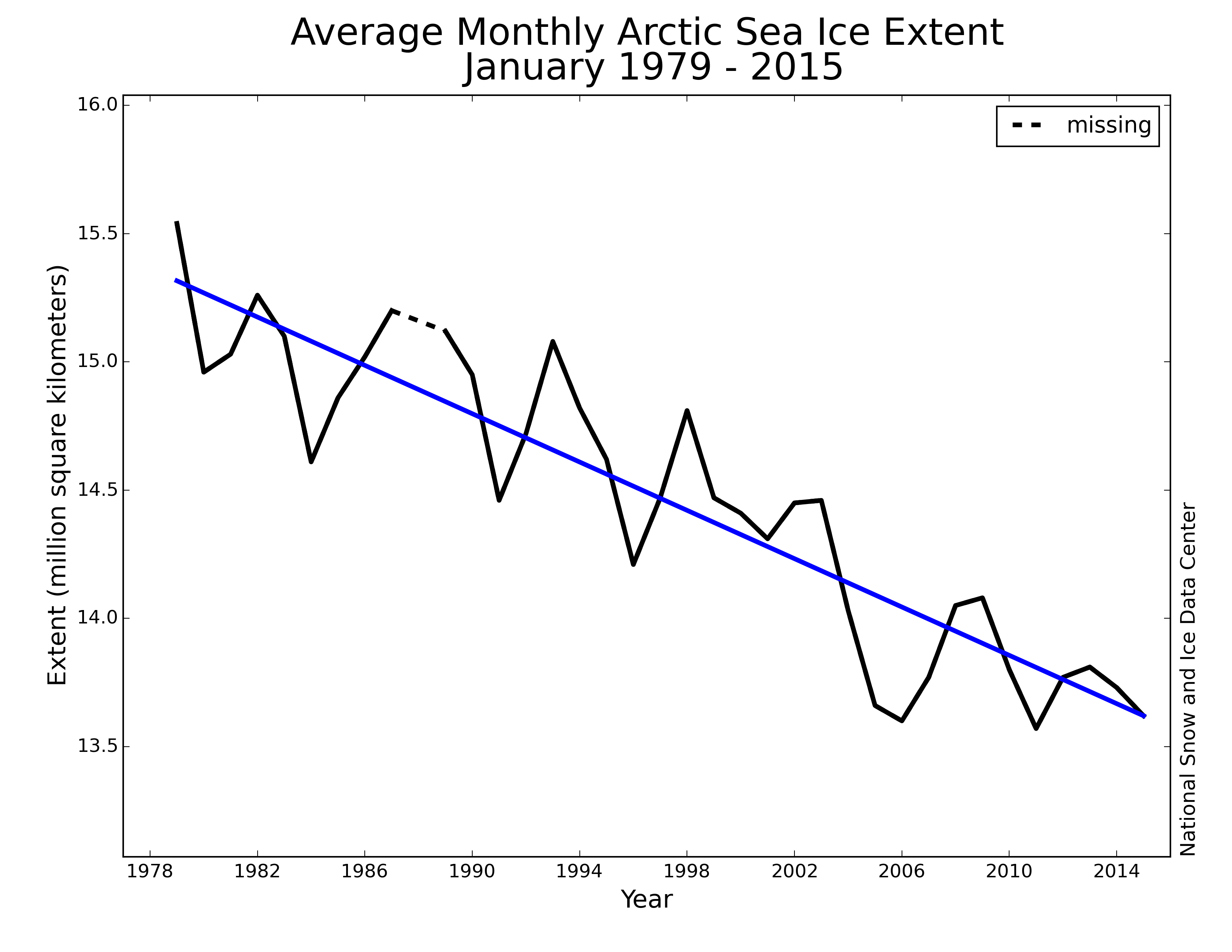
April 2015 compared to previous years

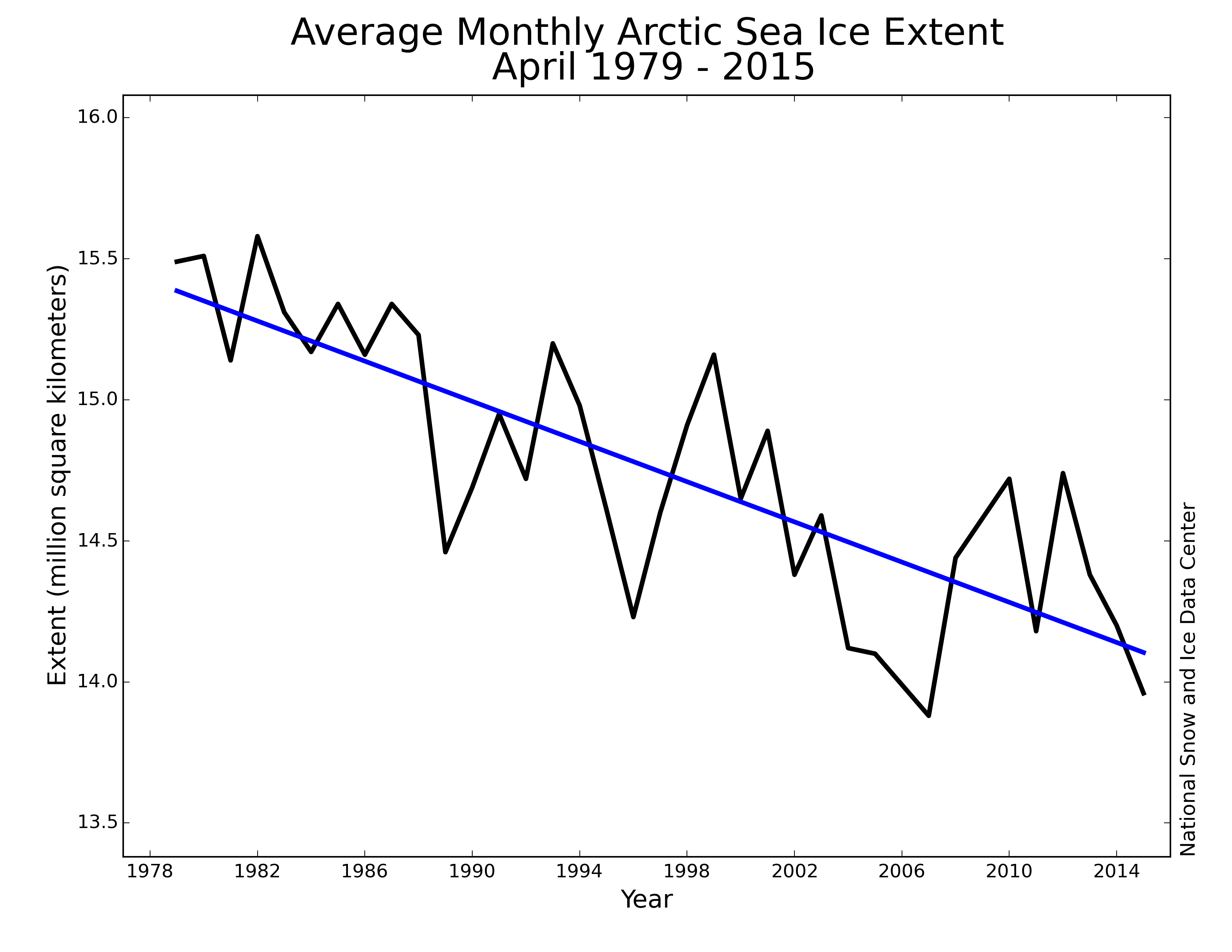
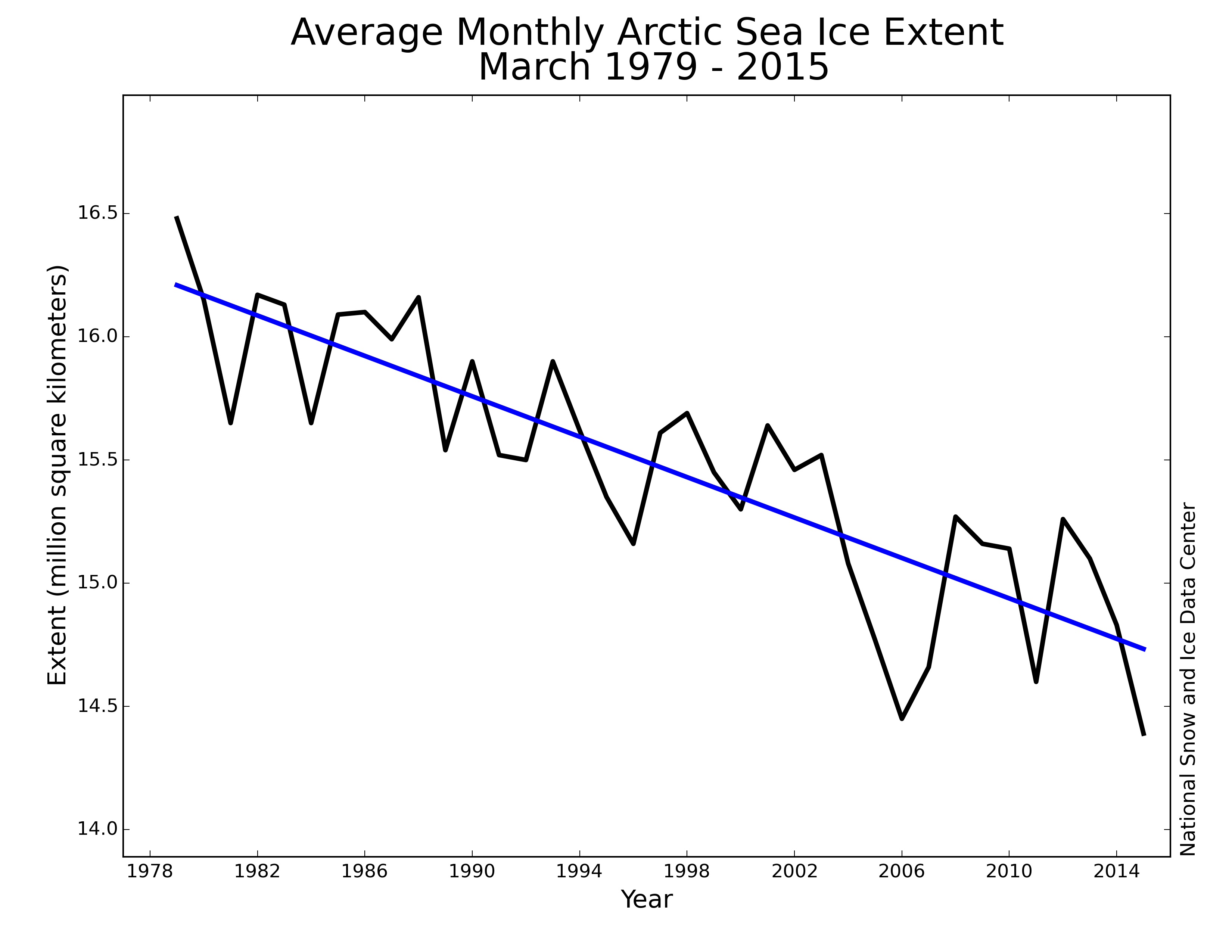
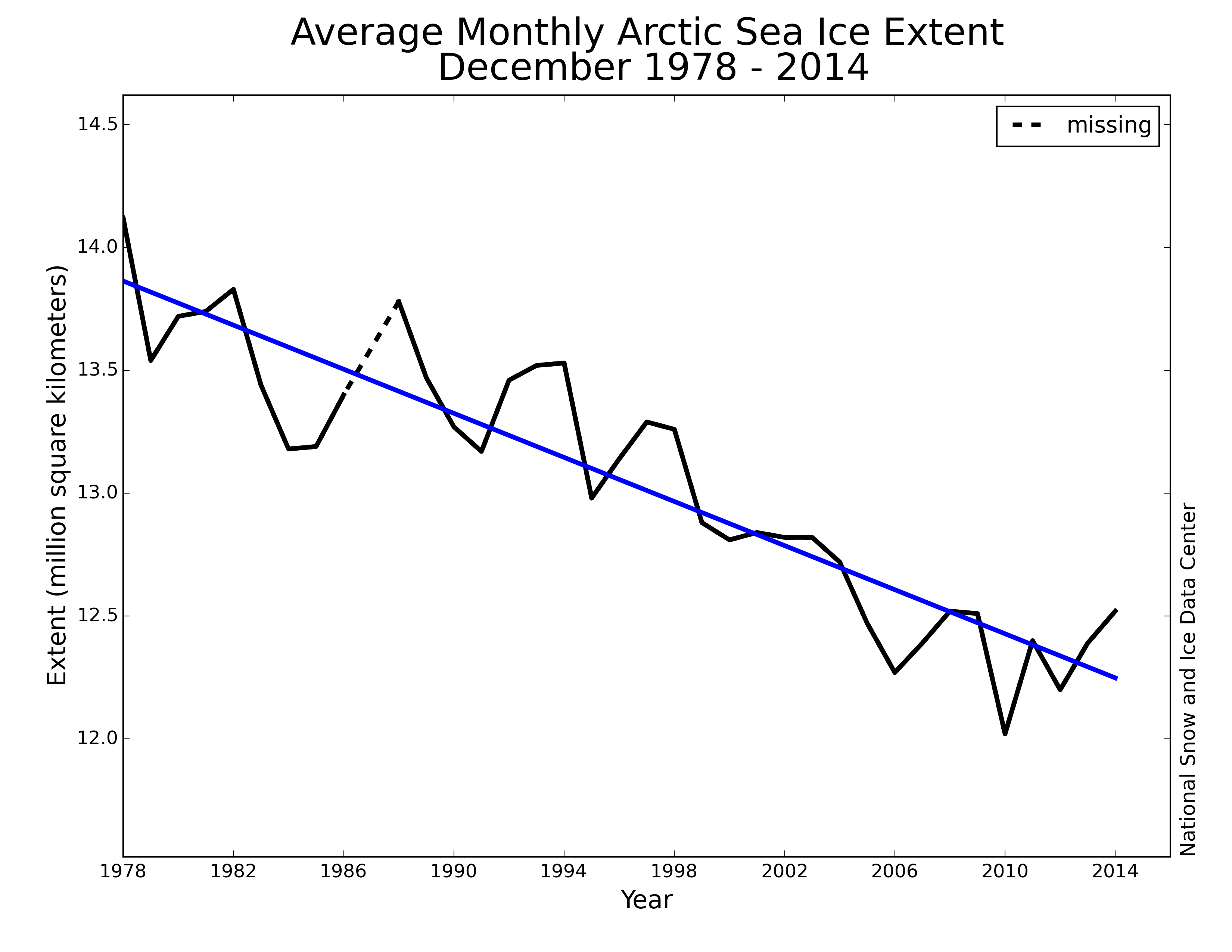
Figure 3. Monthly April ice extent for 1979 to 2015 shows a decline of 2.4% per decade relative to the 1981 to 2010 average.

Credit: National Snow and Ice Data Center
High-resolution image

Arctic sea ice extent averaged for April 2015 was the second lowest in the satellite record for the month. Through 2015, the linear rate of decline for April extent is 2.4% per decade.

New data on sea ice thickness

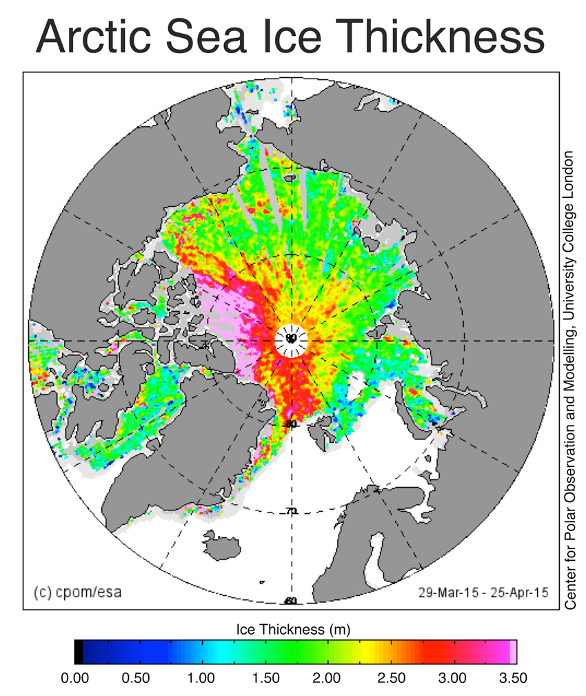
Figure 4. This map shows sea ice thickness in meters in the Arctic Ocean from March 29, 2015 to April 25, 2015.

Credit: Center for Polar Observation and Modelling, University College London
High-resolution image

Data from new sensors, combined with older sources, are providing a more complete picture of ice thickness changes across the Arctic. In a recently published paper, R. Lindsay and A. Schweiger provide a longer-term view of ice thickness, compiling a variety of subsurface, aircraft, and satellite observations. They found that ice thickness over the central Arctic Ocean has declined from an average of 3.59 meters (11.78 feet) to only 1.25 meters (4.10 feet), a reduction of 65% over the period 1975 to 2012.

In addition, near-real-time thickness data from the European Space Agency’s CryoSat-2 satellite are now available from the Centre for Polar Observation and Modelling at the University College London. The spatial pattern of ice thickness in spring is a key factor in the evolution of sea ice through the Arctic summer, and CryoSat-2 data bring the promise of regular sea ice thickness monitoring over most of the Arctic Ocean.

The data indicate that Arctic sea ice thickness in the spring of 2015 is about 25 centimeters (10 inches) thicker than in 2013. Ice more than 3.5 meters (11.5 feet) thick is found off the coast of Greenland and the Canadian Archipelago, and scattered regions of 3-meter (10 feet) thick ice extend across the Beaufort and Chukchi seas. Elsewhere, most of the ice is 1.5 to 2.0 meters (4.9 to 6.6 feet) thick, typical for first-year ice at the end of winter.

Older ice spreads out

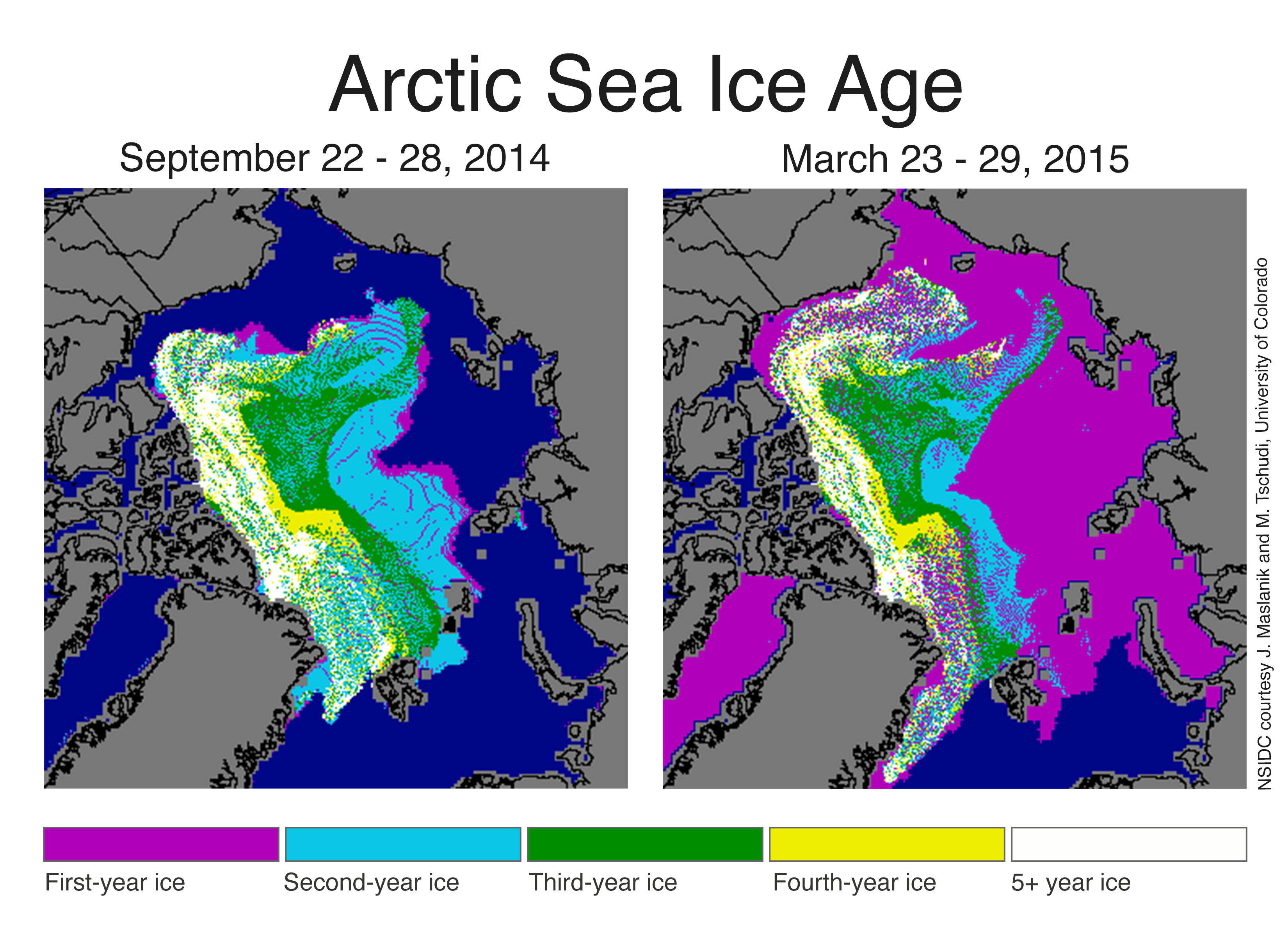
Figure 5. These ice age maps show a change in distribution of older ice from just after the summer 2014 melt season (left) and the end of March 2015 (right).

Credit: NSIDC courtesy J. Maslanik and M. Tschudi, University of Colorado Boulder
High-resolution image

Thickness estimates from CryoSat-2 data and the Lindsay and Schweiger analysis agree well with reconstructions based on sea ice age produced at the University of Colorado Boulder. Since ice gets thicker as it survives several melt seasons, ice age is a good proxy for thickness. For example, the ice thickness map from CryoSat-2 (Figure 4) and the ice age map (Figure 5) both show increased ice thickness in the southern Beaufort Sea where there was a transport of 5+ year old ice this winter. Interestingly, the ice age map identifies the tongue of ice extending towards the New Siberian Islands as second-year ice, yet the ice thickness map shows that its thickness is more similar to first-year ice.

Arctic sea ice age data are now publicly available from NSIDC and can be viewed interactively on the NSIDC Satellite Observations of Arctic Change Web site. Data are currently available through December 2012.

After the 2014 September minimum, first-year ice expanded through the winter growth season and older ice was redistributed around the Arctic Ocean. Figure 5 shows that winds have compressed second-year ice towards the coast of Greenland and the Canadian Archipelago. Old multi-year ice (4+ years old) drifted into the Beaufort and Chukchi seas and spread out, with first-year ice forming between parcels of the older ice. Some of the multi-year ice (both second-year and older) drifted out of the Arctic through Fram Strait on its way to melting in the warm waters of the North Atlantic.

Overall, the area of second-year ice decreased by more than a third during the winter, while ice of four years and more declined by about 10%. In recent years, the Beaufort and Chukchi seas have seen substantial loss of ice during summer, even of the thicker, older ice.

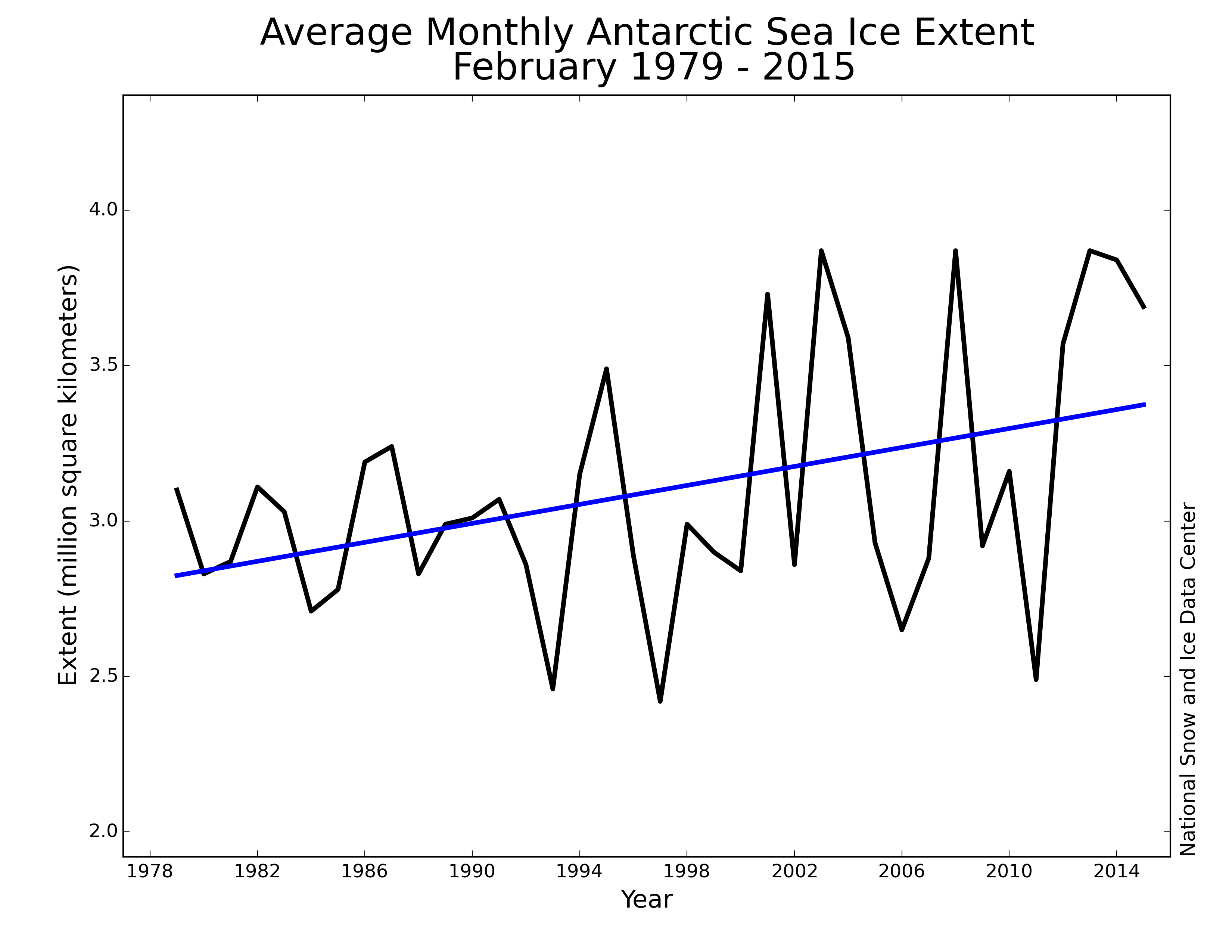
Antarctica reaches record ice extent, but temperature trends vary

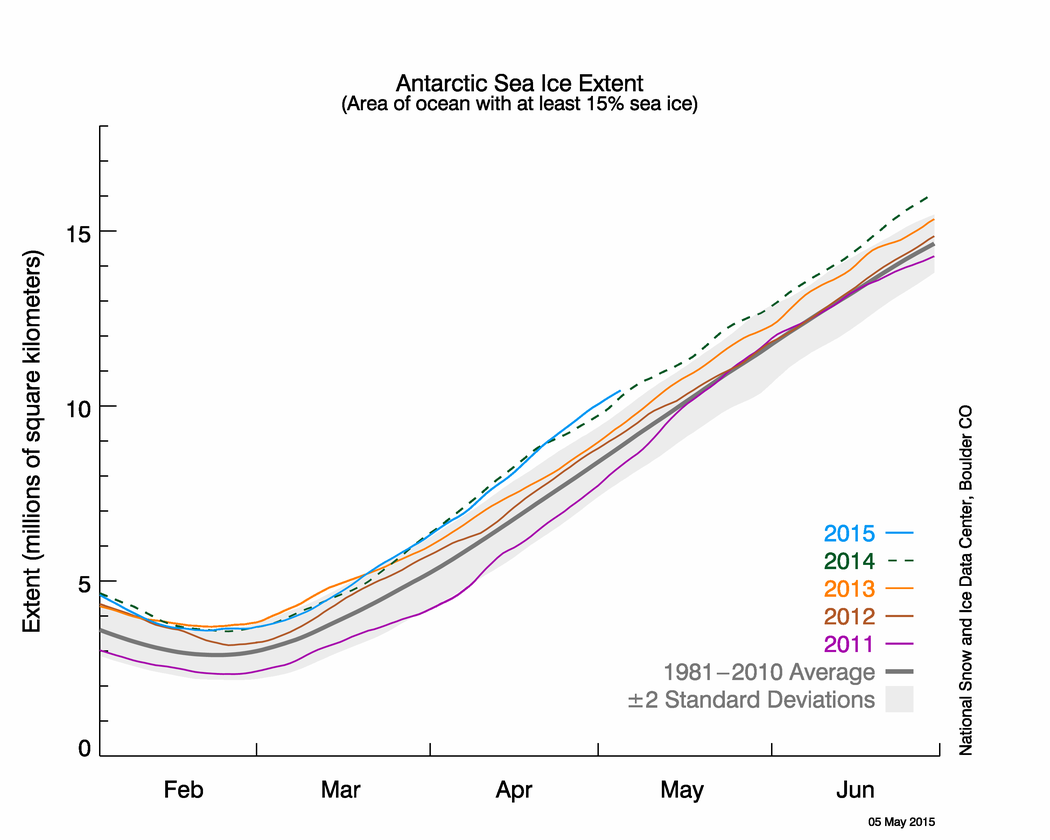
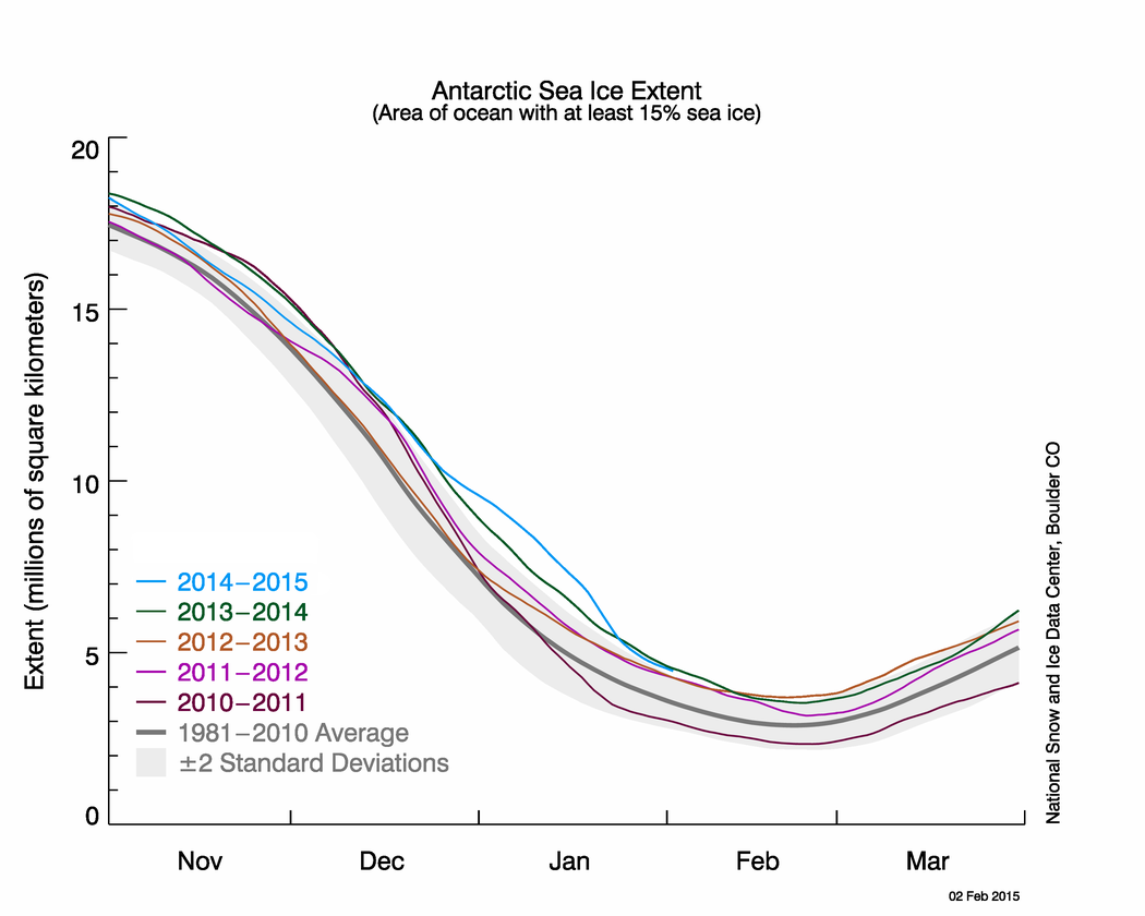
Figure 6. The graph above shows Antarctic sea ice extent as of May 5, 2015, along with daily ice extent data for four previous years. 2015 is shown in blue, 2014 in green, 2013 in orange, 2012 in brown, and 2011 in purple. The 1981 to 2010 average is in dark gray. The gray area around the average line shows the two standard deviation range of the data. Sea Ice Index data.

Credit: National Snow and Ice Data Center
High-resolution image

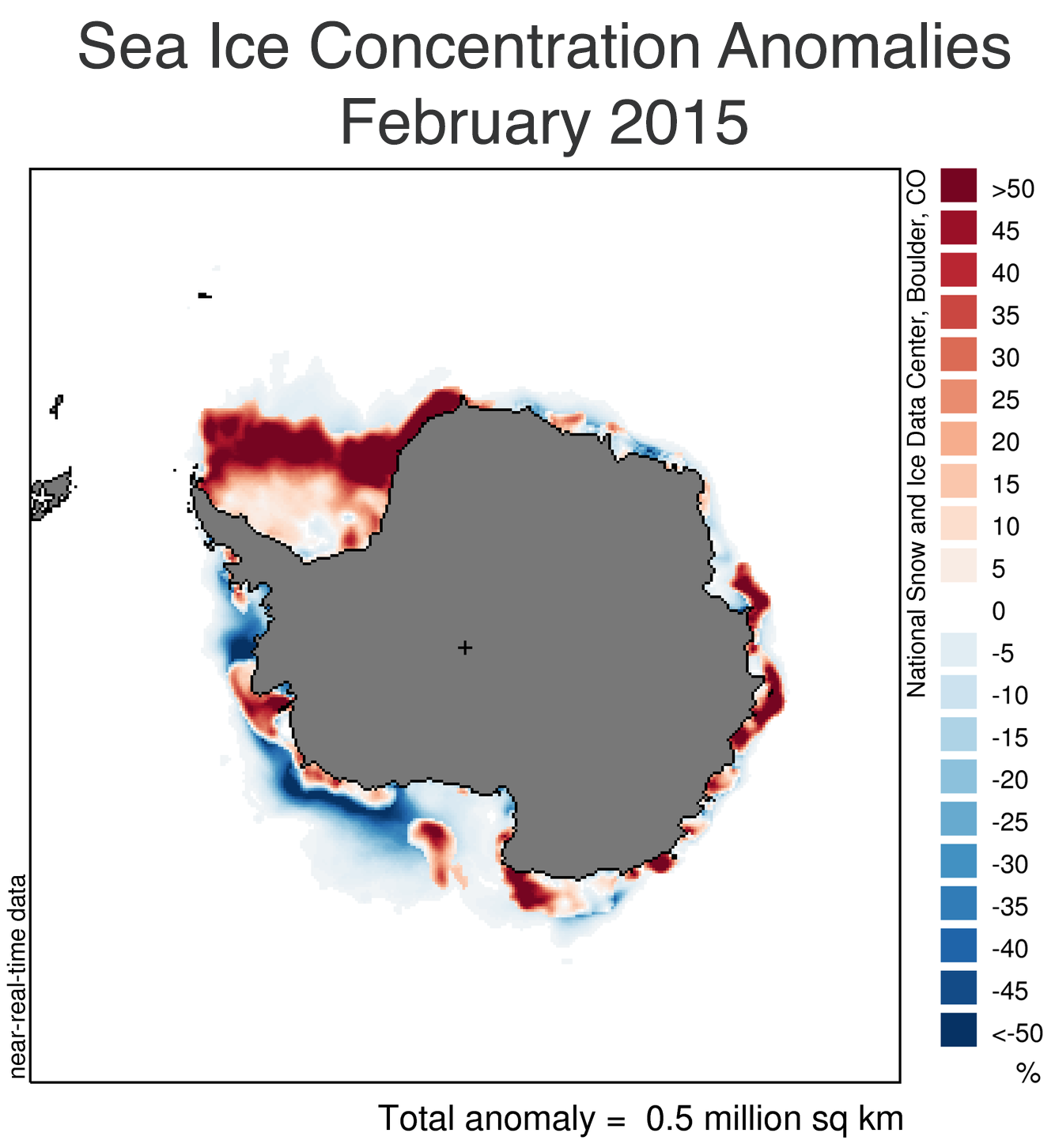
Antarctic sea ice extent averaged 9.06 million square kilometers (3.5 million square miles) for the month and is now the highest April extent in the satellite record. April extent was 300,000 square kilometers (116,000 square miles) higher than the previous record observed in 2014, and 1.70 million square kilometers (656,000 square miles) above the 1981 to 2010 long-term average. The Antarctic April extent was also above the two standard deviations of the long-term average.

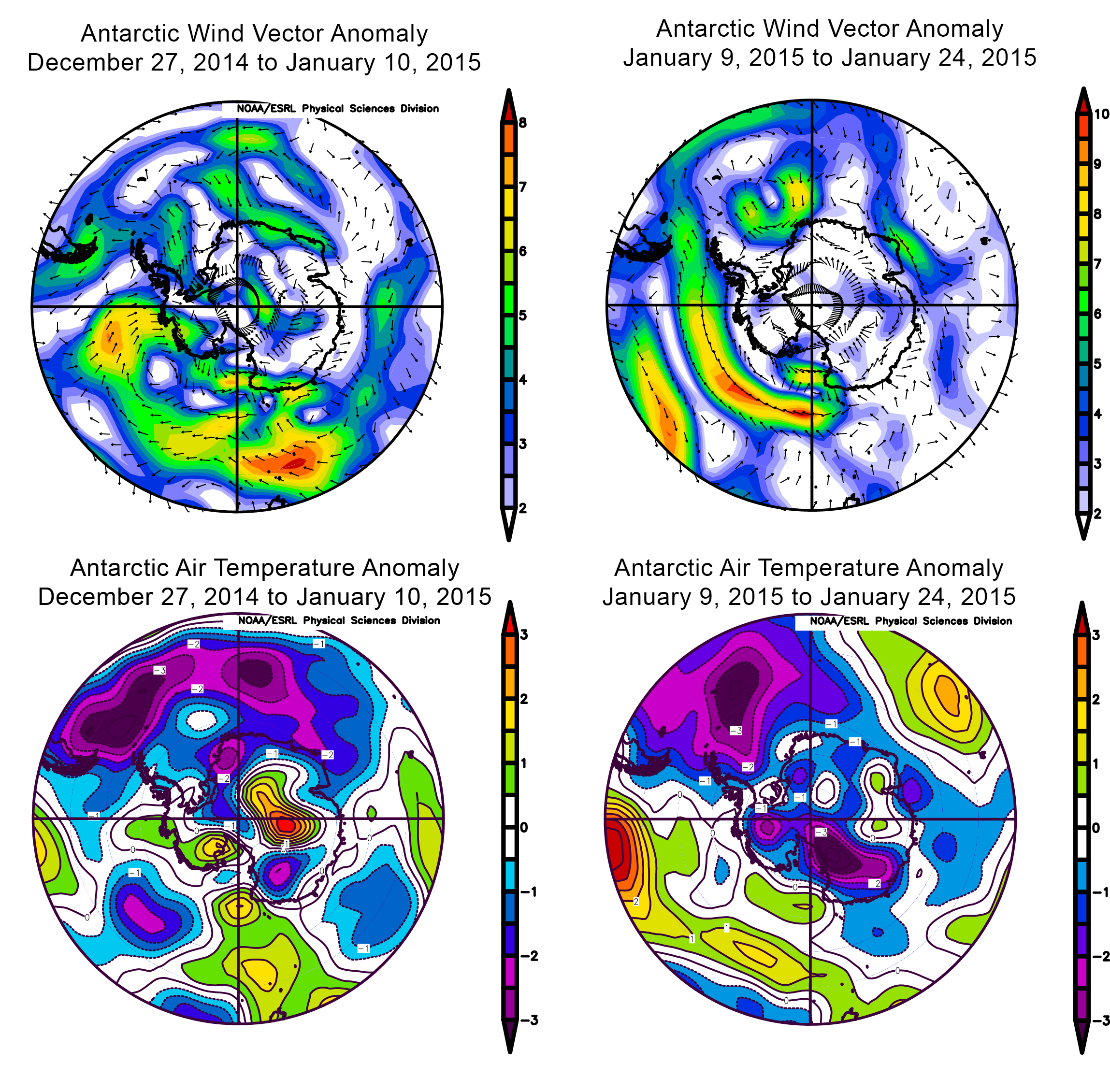
The high sea ice extent in the Antarctic was a result of above-average extent in the Weddell Sea, and slightly more expansive ice cover in the Ross Sea. Interestingly, 925 hPa air temperatures over a wide area in the Weddell Sea were 1 to 4 degrees Celsius (2 to 7 degrees Fahrenheit) above average for the month of April. Lower-than-average air temperatures (1 to 4 degrees Celsius or 2 to 7 degrees Fahrenheit below average) were found in the Ross Sea, but only in the far west and not near the regions of record ice extent. While there remains considerable year-to-year variability of sea ice extent in the Antarctic, the trend in April sea ice extent for the Antarctic from 1979 to 2015 now stands at 4.1% per decade.

References

Lindsay, R. and A. Schweiger. 2015. Arctic sea ice thickness loss determined using subsurface, aircraft, and satellite observations. The Cryosphere, 9, 269-283, doi:10.5194/tc-9-269-2015, 2015.

Tschudi, M., C. Fowler, and J. Maslanik. 2014. EASE-Grid Sea Ice Age. Boulder, Colorado USA: NASA National Snow and Ice Data Center Distributed Active Archive Center, doi:10.5067/1UQJWCYPVX61.

After reaching its seasonal maximum on February 25, the beginning of the melt season was interrupted by late-season periods of ice growth, largely in the Bering Sea, Davis Strait and around Labrador. Near the end of March, extent rose to within about 83,000 square kilometers (32,000 square miles) of the February 25 value. The monthly average Arctic sea ice extent for March was the lowest in the satellite record.

Overview of conditions

Figure 1. Arctic sea ice extent for March 2015 was 14.39 million square kilometers (5.56 million square miles). The magenta line shows the 1981 to 2010 median extent for that month. The black cross indicates the geographic North Pole. Sea Ice Index data. About the data

Credit: National Snow and Ice Data Center
High-resolution image

Arctic sea ice extent for March 2015 averaged 14.39 million square kilometers (5.56 million square miles). This is the lowest March ice extent in the satellite record. It is 1.13 million square kilometers (436,000 square miles) below the 1981 to 2010 long-term average of 15.52 million square kilometers (6.00 million square miles). It is also 60,000 square kilometers (23,000 square miles) below the previous record low for the month observed in 2006.

Conditions in context

Figure 2. The graph above shows Arctic sea ice extent as of April 5, 2015, along with daily ice extent data for four previous years. 2015 is shown in blue, 2014 in green, 2013 in orange, 2012 in brown, and 2011 in purple. The 1981 to 2010 average is in dark gray. The gray area around the average line shows the two standard deviation range of the data. Sea Ice Index data.

Credit: National Snow and Ice Data Center
High-resolution image

The change in total Arctic sea ice extent for March is typically quite small. It tends to increase slightly during the first part of the month, reach the seasonal maximum, and then decline over the remainder of the month. Following the seasonal maximum recorded on February 25, this year instead saw a small decline over the first part of March, and then an increase, due largely to periods of late ice growth in the Bering Sea, Davis Strait and around Labrador. On March 26, extent had climbed to within 83,000 square kilometers (32,000 square miles) of the seasonal maximum recorded on February 25. Despite this late-season ice growth, analysts at the Alaska Ice Program report in their April 3 post that ice in the Bering Sea was very broken up.

March 2015 compared to previous years

Figure 3. Monthly March ice extent for 1979 to 2015 shows a decline of 2.6% per decade relative to the 1981 to 2010 average.

Credit: National Snow and Ice Data Center
High-resolution image

The monthly average Arctic sea ice extent for March was the lowest in the satellite record. Through 2015, the linear rate of decline for March extent is 2.6% per decade.

Overview of the winter season

Figure 4. The plot shows Arctic air temperature anomalies at the 925 hPa level in degrees Celsius for March 2015. Yellows and reds indicate higher than average temperatures; blues and purples indicate lower than average temperatures.

Credit: NSIDC courtesy NOAA Earth System Research Laboratory Physical Sciences Division
High-resolution image

As discussed in our previous post, the winter of 2014/2015 was characterized by an unusual pattern of atmospheric circulation, with the jet stream lying well north of its usual location over Eurasia and the North Pacific, and then plunging southwards over eastern North America. This pattern was associated with unusually warm conditions extending across northern Eurasia, the Bering Sea and Sea of Okhotsk, Alaska and into the western part of the United States, contrasting with cold and snowy conditions over the eastern half of the United States. The record low seasonal maximum in ice extent recorded on February 25, 2015 was largely due to low extent in the unusually warm Bering Sea and Sea of Okhotsk. This pattern of atmospheric circulation and temperatures largely continued through March.

Recent work by Dennis Hartmann of the University of Washington suggests that this unusual jet stream pattern was driven, at least in part, by a particular configuration of sea surface temperatures over the tropical Pacific known as the North Pacific Mode, or NPM. The NPM pattern consists of above-average sea surface temperatures in the western Tropical Pacific that extend north and east towards the California coast and across the far northern Pacific Ocean. While the better-known El-Nino-Southern Oscillation (ENSO) pattern has been in a neutral state for the past few winters, the NPM has been in an extreme positive state since the summer of 2013.

The pattern of air temperatures seen this past winter has persisted through March; note the unusually warm conditions over northern Eurasia, Alaska and western North America, contrasting with unusually cold conditions over eastern North America.

Snow cover update

Figure 5. This map shows the rank of snow water equivalent measured at SNOTEL sites across the western U.S. A rank of 1 (black dots) corresponds to the lowest SWE in the SNOTEL record; a rank of 31 (magenta dots) is the highest.

Credit: Andrew Slater, NSIDC
High-resolution image

The unusual atmospheric circulation pattern just discussed also helps to explain the snow drought over the western United States. NSIDC scientist Andrew Slater maintains regular updates of western U.S. mountain snowpack conditions using data from the SNOTEL (snowpack telemetry) system – a network of automated sensors that measure snow water equivalent. The automated SNOTEL sites are complemented by snowcourses, where snow water equivalent is measured manually on a periodic basis.

Typically, the snowpack peaks around April 1. As seen in Figure 5, the April 1 snowpack over most of the western United States is far below average. At many sites, snow water equivalent is at historic lows for this time of year. Conditions are somewhat better along the Front Range of Colorado and in Arizona, Wyoming and Montana.

Record warmth in Antarctica

Air temperatures reached record high levels at two Antarctic stations last week, setting a new mark for the warmest conditions ever measured anywhere on the continent. On March 23, at Argentina’s base Marambio, a temperature of 17.4° Celsius (63.3° Fahrenheit) was reached, surpassing a previous record set in 1961 at a nearby base, Esperanza. The old record was 17.1° Celsius (62.8° Fahrenheit). However, Esperanza quickly reclaimed the record a few hours later on March 24, reaching a temperature of 17.5° Celsius (63.5° Fahrenheit).

The cause of these warm conditions is familiar to people living in mountainous regions: a foehn or chinook wind, in which air flows up and over a steep mountain ridge. On the windward side, moisture is wrung out of the air mass in the form of rain or snow. As the air descends on the leeward (downwind) side, it compresses and warms.

This airflow pattern is a key part of the climate conditions that led to past ice shelf disintegrations in the region, such as the dramatic break-up of the Larsen B Ice Shelf in 2002. Air pressure patterns during the event indicated a near-stationary high pressure center in the Drake Passage north of the Antarctic Peninsula, and a strong area of low pressure at the base of the Peninsula, favoring the foehn pattern. Events like this have been recorded by a network of sensors installed by the National Science Foundation LARISSA project.  This network recorded temperatures as high as 16.9° Celsius (62.4° Fahrenheit), westerly winds up to 23 meters per second (45 miles per hour), and a ~100 hour period of temperatures above freezing over the Larsen B area. A recent publication by a colleague at the Scripps Institute of Oceanography describes the impact of foehn or chinook patterns on ice shelf and sea ice stability in the region, making use of the network of Automated Meteorology-Ice-Geophysics Observing Systems (AMIGOS) and other weather sensors in the region.

Further reading

Cape, M., M. Vernet, P. Skvarca, S. Marinsek, T. Scambos, and E. Domack. 2015. Foehn winds link climate-driven warming to coastal cryosphere evolution in Antarctica. Jour. Geophys. Res., Atmospheres, submitted.

Scambos, T., R. Ross, T. Haran, R. Bauer, D.G. Ainley, K.-W. Seo, M. Keyser, A. De, Behar, D.R. MacAyeal. 2013. A camera and multisensor automated station design for polar physical and biological systems monitoring: AMIGOS. Journal of Glaciology, 59 (214), 303-314, doi: 10.3189/2013JoG12J170.

Arctic sea ice extent continues to track well below average, but it is still unclear whether March will see an increase in ice, or establish a record low maximum. Regionally, Arctic ice extent is especially low in the Sea of Okhotsk and the Bering Sea. In the Antarctic, sea ice shrank to the fourth highest minimum in the satellite record.

Overview of conditions

Figure 1. Arctic sea ice extent for February 2015 was 14.41 million square kilometers (5.56 million square miles). The magenta line shows the 1981 to 2010 median extent for that month. The black cross indicates the geographic North Pole. Sea Ice Index data. About the data

Credit: National Snow and Ice Data Center
High-resolution image

Arctic sea ice extent in February averaged 14.41 million square kilometers (5.56 million square miles). This is the third lowest February ice extent in the satellite record. It is 940,000 square kilometers (362,900 square miles) below the 1981 to 2010 long-term average of 15.35 million square kilometers (5.93 million square miles). It is also 50,000 square kilometers (19,300 square miles) above the record low for the month observed in 2005.

With the Arctic Ocean completely ice covered, the remaining areas of potential new ice growth are limited to the margins of the pack in the northern Pacific and northern Atlantic. Sea ice extent is below average across the entire sea ice margin, most prominently along the Pacific sectors. A small region of above-average ice extent is located near Newfoundland and the Canadian Maritime Provinces.

The Arctic maximum is expected to occur in the next two or three weeks. Previous years have seen a surge in Arctic ice extent during March (e.g., in 2012, 2014). However, if the current pattern of below-average extent continues, Arctic sea ice extent may set a new lowest winter maximum.

Conditions in context

Figure 2. The graph above shows Arctic sea ice extent as of March 2, 2015, along with daily ice extent data for four previous years. 2014 to 2015 is shown in blue, 2013 to 2014 in green, 2012 to 2013 in orange, 2011 to 2012 in brown, and 2010 to 2011 in purple. The 1981 to 2010 average is in dark gray. The gray area around the average line shows the two standard deviation range of the data. Sea Ice Index data.

Credit: National Snow and Ice Data Center
High-resolution image

Arctic sea ice extent increased by 429,000 square kilometers (165,600 square miles) during the month of February. This gain was slightly less than the average for the month. While low extent for the Arctic as a whole was largely driven by conditions in the Sea of Okhotsk and the Bering Sea, extent was also slightly below average along the Barents Sea and parts of the East Greenland Sea.

February 2015 compared to previous years

Figure 3. Monthly February ice extent for 1979 to 2015 shows a decline of 2.9% per decade relative to the 1981 to 2010 average.

Credit: National Snow and Ice Data Center
High-resolution image

The monthly average Arctic sea ice extent for February was the third lowest in the satellite record. Through 2015, the linear rate of decline for February extent is 2.9% per decade.

Hot Bering(s)

Figure 4. The plot shows Arctic air temperature anomalies at the 925 hPa level in degrees Celsius for February 2015. Yellows and reds indicate higher than average temperatures; blues and purples indicate lower than average temperatures.

Credit: NSIDC courtesy NOAA Earth System Research Laboratory Physical Sciences Division
High-resolution image

The low ice extent in the Bering Sea and Sea of Okhotsk is linked to unusually warm conditions in the area. February air temperatures at the 925 hPa level were as much as 4 to 6 degrees Celsius (7 to 11 degrees Fahrenheit) above average in the northern Bering Sea, easternmost Siberia, and Sea of Okhotsk.

While these localized hotspots are in part driven by the low sea ice extent and the resulting large heat fluxes from the open water to the atmosphere, they are seen to be part of a broad area of unusually warm conditions extending across most of northern Eurasia, across Alaska, and into the western part of the United States. In contrast, cold and snowy conditions have persisted across the eastern half of North America. Broadly speaking, these opposing patterns of warmth and cold, along with low ice extent in the Sea of Okhotsk and Bering Sea, can be linked to an unusual jet stream pattern, with the jet lying north of its usual location over Eurasia and the North Pacific (meaning that warm air extends further north than is usual), and then plunging southwards over eastern North America.

Snow cover

Figure 5a. This snow cover anomaly map shows the difference between snow cover for February 2015, compared with average snow cover for February from 1981 to 2010. Areas in orange and red indicate lower than usual snow cover, while regions in blue had more snow than normal.

Credit: National Snow and Ice Data Center, courtesy Rutgers University Global Snow Lab
High-resolution image

Figure 5b. This graphs shows snow cover extent anomalies in the Northern Hemisphere for February from 1967 to 2015. The anomaly is relative to the 1981 to 2010 average.

Credit: National Snow and Ice Data Center, courtesy Rutgers University Global Snow Lab
High-resolution image

This unusual jet stream pattern is clearly manifested in the pattern of Northern hemisphere snow cover for February. Snow extent was well above average over the northeastern U.S. However, the western U.S. and Northern Rockies saw less snow cover than average, especially along the Pacific coast where it has been particularly warm and severely dry. While the Tibetan Plateau saw a somewhat more extensive snow cover than average in December and January, extent for Tibet and Eurasia as a whole was below average in February. Higher-than-average snow cover in the eastern U.S. expanded and became more pronounced this month as well. All of these are continuations of the basic pattern seen in December and January, although the pattern of extensive snow over the northeastern U.S. became more pronounced this month. The low snow cover extent in much of Eurasia is consistent with the warmer-than-average conditions there as described above.

Seasonal Antarctic minimum reached

Figure 6a. This figure shows the concentration anomaly for February 2015 monthly average extent relative to the 1981 to 2010 average. Sea Ice Index data. About the data

Credit: National Snow and Ice Data Center
High-resolution image

Figure 6b. Monthly Antarctic February ice extent for 1979 to 2015 shows a trend of 5.0% per decade relative to the 1981 to 2010 average.

Credit: National Snow and Ice Data Center
High-resolution image

Antarctic sea ice extent reached its annual minimum, dipping to 3.58 million square kilometers (1.38 million square miles) on February 20. This is the fourth highest summer minimum extent on record, trailing behind 2008 (3.75 million square kilometers or 1.44 million square miles, highest), 2013, and 2003. The 2014 Antarctic minimum ranked the fifth highest (3.54 million square kilometers or 1.36 million square miles). For the month as a whole, February 2015 has the sixth highest ice extent (3.8 million square kilometers or 1.46 million square miles). The sea ice extent trend for February for 1979 to 2015 shows an increase of 5.0%  per decade. However, Antarctica’s sea ice extent is highly variable. As recently as 2011, Antarctic sea ice extent was at near-record low levels for the summer minimum.

Nevertheless, the recent series of high-ice-extent minima is part of a remarkable recent uptick in extent year-round for Antarctica, dominated by extensive ice in both the Weddell Sea (south of Africa) and the Ross Sea (south of New Zealand). Sea ice in the eastern Weddell Sea presently extends several hundred kilometers further north and east of its typical extent, while ice extent in the Ross Sea is presently near average. The debate continues regarding the cause of the recent Antarctic trends, but the best explanation so far involves a combination of strengthening low pressure in the eastern Ross Sea (the Amundsen Sea Low) and the eastern Weddell Sea, and a persistently positive phase of the Southern Annular Mode. The freshening of surface seawater around Antarctica may also play a role.

Global sea ice trends

Claire Parkinson of NASA recently presented the global average (Arctic plus Antarctic) trend in sea ice extent for the period 1979 to 2013. Overall, global sea ice has declined, despite the positive trend in Antarctic extent. The annual average trend is -35,000 square kilometers (-13,500 square miles) per year, or about -1.5% per decade. The strong Arctic decline in September leads to the largest magnitude monthly trend for global sea ice in that month, at -68,000 square kilometers (-26,300 square miles) per year, or -2.6% per decade. See the NSIDC FAQ on global sea ice here.

Further reading

Parkinson, C. L. 2014. Global sea ice coverage from satellite data: annual cycle and 35-year trends. Journal of Climate, doi: 10.1175/JCLI-D-14-00605.1.

Arctic sea ice extent was the third lowest for the month of January. Ice extent remained lower than average in the Bering Sea and Sea of Okhotsk, while ice in the Barents Sea was near average. Antarctic sea ice extent declined rapidly in late January, but remains high.

Overview of conditions

Figure 1. Arctic sea ice extent for January 2015 was 13.62 million square kilometers (5.26 million square miles). The magenta line shows the 1981 to 2010 median extent for that month. The black cross indicates the geographic North Pole. Sea Ice Index data. About the data

Credit: National Snow and Ice Data Center
High-resolution image

Sea ice extent in January averaged 13.62 million square kilometers (5.26 million square miles). This is 910,000 square kilometers (351,000 square miles) below the 1981 to 2010 long-term average of 14.53 million square kilometers (5.61 million square miles), and 50,000 square kilometers (19,000 square miles) above the record low for the month observed in 2011.

This below-average Arctic extent is mainly a result of lower-than-average extent in the Bering Sea and the Sea of Okhotsk. On the Atlantic side, Barents Sea ice extent is near average. This is in sharp contrast to the general pattern seen since 2004 of below average extent in this region, but above average extent in the Bering Sea. Ice extent is also near average in the East Greenland Sea, Baffin Bay and the Labrador Sea.

Conditions in context

Figure 2. The graph above shows Arctic sea ice extent as of February 2, 2015, along with daily ice extent data for four previous years. 2014 to 2015 is shown in blue, 2013 to 2014 in green, 2012 to 2013 in orange, 2011 to 2012 in brown, and 2010 to 2011 in purple. The 1981 to 2010 average is in dark gray. The gray area around the average line shows the two standard deviation range of the data. Sea Ice Index data.

Credit: National Snow and Ice Data Center
High-resolution image

During most of January, the Arctic Oscillation (AO) was in a strongly positive phase. When the AO is in a positive phase, sea level pressure in the Arctic is particularly low, and sea level pressure is relatively high in the middle latitudes of the Northern Hemisphere. Variability in Arctic sea ice conditions is strongly influenced by the phase of the AO. Typically, during the positive phase of the AO, surface winds push ice away from the shores of Siberia, leading to the formation of more young, thin ice that is prone to melting out in summer. The positive phase also tends to increase the transport of thick, multiyear ice out of the Arctic through Fram Strait.

Air temperatures (at the 925 millibar level, about 3,000 feet above the surface) were mostly above average over most of the Arctic Ocean, with positive anomalies of 4 to 6 degrees Celsius (7 to 11 degrees Fahrenheit) over the Chukchi and Bering seas on the Pacific side of the Arctic, and also over the East Greenland Sea on the Atlantic side.

January 2015 compared to previous years

Figure 3. Monthly January ice extent for 1979 to 2015 shows a decline of 3.2% per decade relative to the 1981 to 2010 average.

Credit: National Snow and Ice Data Center
High-resolution image

Arctic sea ice extent for January was the third lowest in the satellite record. Through 2015, the linear rate of decline for January extent over the satellite record is 3.2% per decade.

Barents Sea ice variability

Figure 4. The graph shows Barents Sea ice area (blue line) and ocean temperatures in the Barents Sea Opening (red line) from 1980 to 2015. The sea ice area tends to be smaller for higher Atlantic water temperatures, with a lag of 1 to 2 years (note the reversed scale for Atlantic water temperatures). The data are based on Årthun et al. (2012), who find that the ocean temperature largely reflects changes in volume of Atlantic water inflow. Sea ice area anomalies are from the NASA Team algorithm (Cavalieri et al., 1996), provided by the National Snow and Ice Data Center. Ocean temperature has been sampled by the Institute of Marine Research (IMR), Norway, and is a section between Norway and Bear Island (BSO; 71.5-73.5N, 20E).

Credit: Ingrid Onarheim, Bjerknes Centre for Climate Research
High-resolution image

Variability in winter sea ice in the Barents Sea largely reflects ocean heat transport. The inflow of Atlantic water between Norway and Bear Island (the Barents Sea Opening or BSO) is the Barents Sea’s main oceanic heat source. Because there are no significant freshwater sources reaching the central Barents Sea, this warm Atlantic water extends to the surface and readily impacts the sea ice. This contrasts with the rest of the Arctic Ocean, where the Atlantic water lies well beneath the slightly fresher polar surface layer. The import of sea ice in the northern straits is also small, around 20% of the sea ice area exported southwards in the Fram Strait, meaning that the Barents Sea primarily consists of thin, first-year ice. Thus, periods with large volumes of warm Atlantic water entering into the Barents Sea are correlated with less sea ice formation and overall less sea ice extent.

Variations in winter ice extent in the Barents Sea are well correlated with variations in overall Arctic sea ice extent, as assessed over the satellite record. This winter is an exception. Sea ice extent in the Barents Sea is fairly high compared to recent years, while it is low for the Arctic as a whole. According to colleagues at the University of Bergen, this is due to a reduced overall inflow of Atlantic waters. A maximum in the ocean heat transport occurred in the mid 2000s, yet since then, the inflow has in general lessened, both along the Norwegian coast, through the Fram Strait, and through the Barents Sea Opening between Norway and Bear Island. Variations in Atlantic inflow is a focus of ongoing research at the Bjerknes Centre in Bergen, as well as in other research centers in Europe.

Antarctic sea ice declines rapidly, still high

Figure 5a. The graph above shows Antarctic sea ice extent as of February 2, 2015, along with daily ice extent data for four previous years. 2014 to 2015 is shown in blue, 2013 to 2014 in green, 2012 to 2013 in orange, 2011 to 2012 in brown, and 2010 to 2011 in purple. The 1981 to 2010 average is in dark gray. The gray area around the average line shows the two standard deviation range of the data. Sea Ice Index data.

Credit: National Snow and Ice Data Center
High-resolution image

Antarctic sea ice extent reached record high levels for late December 2014 and early January 2015, peaking around January 10 at more than 2.5 million square kilometers (965,000 square miles) above the 1981 to 2010 average, and 1.05 million square kilometers (580,000 square miles) above the previous record (2014) for that date. As noted last month, the largest excursions are occurring in the northern Weddell Sea and the northern Ross Sea. After January 10, and particularly after January 19, sea ice extent dropped rapidly (~250,000 square kilometers, or 96,500 square miles, per day), and large areas of the northern Ross Sea became ice free. The northern Weddell region still has a very large ice extent relative to average conditions.

Figure 5b. These images show Antarctic wind vector (top) and air temperature (bottom) anomalies for late December 2014 to early January 2015, compared to 1981 to 2010 averages.

Credit: NOAA ESRL Physical Sciences Division
High-resolution image

Weather conditions during late December and January help to explain these changes. In the northern Weddell Sea, southerly winds (more so than average) and cool conditions relative to the 1981 to 2010 average prevailed for late December and all of January, and sea ice there remained high relative to long-term averages for the month. For the northern Ross Sea, air temperatures at the 925 hPa level have been slightly above average for the entire period, but winds in this area shifted during January, from southerly (pushing ice outward) to northwesterly. The combination of northerly winds and slightly warm conditions seems to have reduced the ice extent anomaly significantly in this sector.

Further reading

Smedsrud, L.H., I. Esau, R. B. Ingvaldsen, T. Eldevik, P. M. Haugan, C. Li, V. S. Lien, A. Olsen, A. M. Omar, O. H. Otterå, B. Risebrobakken, A. B. Sandø, V. A. Semenov, and S. A. Sorokina. 2013. The role of the Barents Sea in the Arctic climate system.
Reviews of Geophysics, 51, doi:10.1002/rog.20017.

Årthun, M., T. Eldevik, L. H. Smedsrud, Ø. Skagseth, and R. B. Ingvaldsen. 2012.
Quantifying the Influence of Atlantic Heat on Barents Sea Ice Variability and Retreat. Journal of Climate, Volume 25, pp. 4736-4743, doi:10.1175/JCLI-D-11-00466.1.

Schauer, U. and A. Beszczynska-Möller. 2009. Problems with estimation and interpretation of oceanic heat transport – conceptual remarks for the case of Fram Strait in the Arctic Ocean, Ocean Sci., 5, 487–494.

Arctic sea ice extent remained about a standard deviation below average for the month of December. Compared to recent years, 2014 as a whole was rather unremarkable. The bigger story was the record high extents observed in the Antarctic through more than half of the year. At year’s end, Antarctic sea ice extent was again at a record high, but poised for a rapid decline as the austral summer wears on.

Overview of conditions

Figure 1. Arctic sea ice extent for December 2014 was 12.52 million square kilometers (4.83 million square miles). The magenta line shows the 1981 to 2010 median extent for that month. The black cross indicates the geographic North Pole. Sea Ice Index data. About the data

Credit: National Snow and Ice Data Center
High-resolution image

Sea ice extent in December averaged 12.52 million square kilometers (4.83 million square miles). This is 540,000 square kilometers (208,495 square miles) below the 1981 to 2010 long-term average of 13.06 million square kilometers (5.04 million square miles) and 500,000 square kilometers (193,051 square miles) above the record low for the month observed in 2010.

Both Hudson Bay and Baffin Bay are now essentially completely ice covered. On the Atlantic side, recent winters have been characterized by reduced winter ice extent in the Kara and Barents seas. This is not the case for the winter of 2014 to 2015.

The only two regions where extent is notably below average are in the Bering Sea and the Sea of Okhotsk. This contrasts with recent winters when ice extent has been greater than average in the Bering Sea.

Conditions in context

Figure 2. The graph above shows Arctic sea ice extent as of January 4, 2015, along with daily ice extent data for four previous years. 2014 to 2015 is shown in blue, 2013 to 2014 in green, 2012 to 2013 in orange, 2011 to 2012 in brown, and 2010 to 2011 in purple. The 1981 to 2010 average is in dark gray. The gray area around the average line shows the two standard deviation range of the data.Sea Ice Index data.

Credit: National Snow and Ice Data Center
High-resolution image

Sea ice extent grew 2.00 million square kilometers (772,000 square miles) during the month of December. This was about average for the month. Throughout the month, daily extents were about one standard deviation below 1981 to 2010 averages. This occurred despite the fairly warm conditions over the Eurasian side of the Arctic Ocean. As averaged over the month, air temperatures at the 925 hPa level in the Laptev and East Siberian seas were up to 5 degrees Celsius (9 degrees Fahrenheit) above average, linked to a region of unusually high pressure in the region that led to southerly winds.

December 2014 compared to previous years

Figure 3. Monthly December ice extent for 1979 to 2014 shows a decline of 3.4% per decade relative to the 1981 to 2010 average. The dashed line indicates a period of missing data from December 2, 1987 through January 12, 1988.

Credit: National Snow and Ice Data Center
High-resolution image

Arctic sea ice extent for December was the ninth lowest in the satellite record. Through 2014, the linear rate of decline for December extent over the satellite record is 3.4% per decade.

2014 in review

Compared to recent years, sea ice conditions observed throughout 2014 were largely unremarkable. Throughout the year, extent for the Arctic as a whole remained below average, but generally within two standard deviations of the average. The maximum extent observed on March 21 of 14.91 million square kilometers (5.76 million square miles) was the fifth lowest in the satellite record, with the minimum extent observed on September 17 of 5.02 million square kilometers (1.94 million square miles) being the sixth lowest on record. One event of note was in the Laptev Sea, where during August, open water was observed to extend to about 85 degrees latitude, less than 560 kilometers (350 miles) from the North Pole.

Summer weather conditions, which are known to strongly influence September minimum ice extent, were also largely unremarkable in 2014. Compared to the long term (1981 to 2010) climatology, sea level pressure over the period June through August 2014 was higher than average over much of the central Arctic Ocean, the Atlantic sector of the Arctic, and Greenland. While air temperatures at the 925 hPa level (approximately 3,000 feet altitude) were slightly above average over part of the central Arctic Ocean, they were below average over the Kara Sea and just north of Alaska.

By sharp contrast, sea ice in Antarctica was at satellite-era record high daily levels for much of 2014. On September 22, 2014, Antarctic ice extent reached 20.11 million square kilometers (7.76 million square miles). This was the first year in the modern satellite record that Antarctic ice extent climbed above 20 million square kilometers (7.72 million square miles).

As the year drew to a close, sea ice extent again reached record high levels for the date by declining far more slowly than usual. Extent anomalies are particularly large in the Ross Sea and Amundsen Sea regions, and in the northern Weddell Sea—areas that have been anomalously high for most of the calendar year. However, sea ice concentration in both these regions is now quite low, that is, the sea ice pack is loose and open. This is characteristic of dispersal of the ice by storms, and indeed strong low pressure anomalies were present in the eastern Ross Sea and northern Weddell Sea in the second half of December. The extent of this loose sea ice pack far to the north makes it likely that a rapid decline will occur as warmer summer weather arrives.

Losing the memory of low extent

Figure 4. This graph shows future projections of September sea ice extent under various future greenhouse gas emission levels. Limiting the warming in 2100 to about 1 to 2 degrees Celsius (2 to 4 degrees Fahrenheit) under the RCP2.6 emission scenario would help to stabilize ice conditions at levels seen today. The RCP8.5 emission scenario (warming by about 4 degrees Celsius 0r 7 degrees Fahrenheit by the end of this century) would result in a seasonally ice-free Arctic by the end of this century.

Credit: Julienne Stroeve
High-resolution image

In September of 2014, the Royal Society of London held a workshop focused on the reduction in Arctic sea ice extent. One outcome of this meeting was a greater understanding of the overall trajectory of September ice extent. In a nutshell, it appears that very large departures from the overall downward trend in September extent are unlikely to persist into the following September. If a given September has very low ice extent, strong winter heat loss results in strong ice growth, so that the “memory” of the low ice September ice extent is lost. If a given September has a high ice extent, winter heat loss is more limited, meaning less ice growth. Consequently, while there can be large departures from year to year from the downward linear trend in ice extent (e.g., September 2012 compared to 2014), the natural tendency is for the large departure to dampen out, so that, overall, ice extent stays on the long-term downward trajectory that will eventually lead to seasonally ice free conditions as the Arctic continues to warm in response to rising atmospheric concentrations of Greenhouse gases.