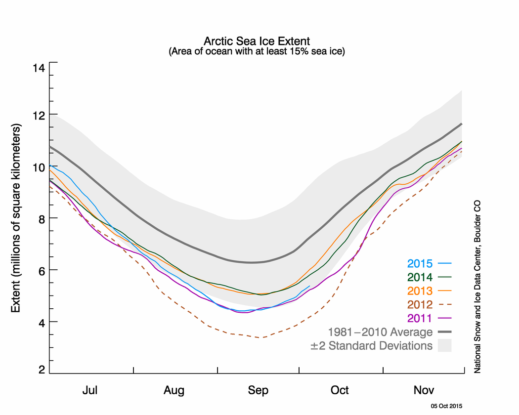
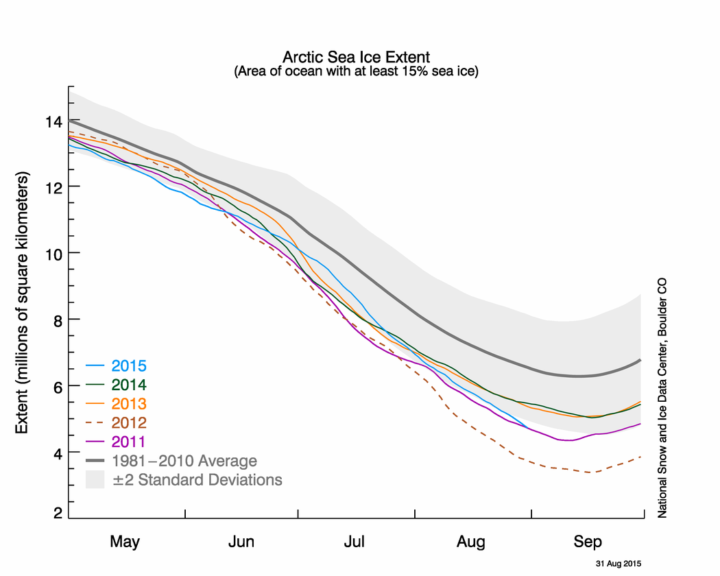
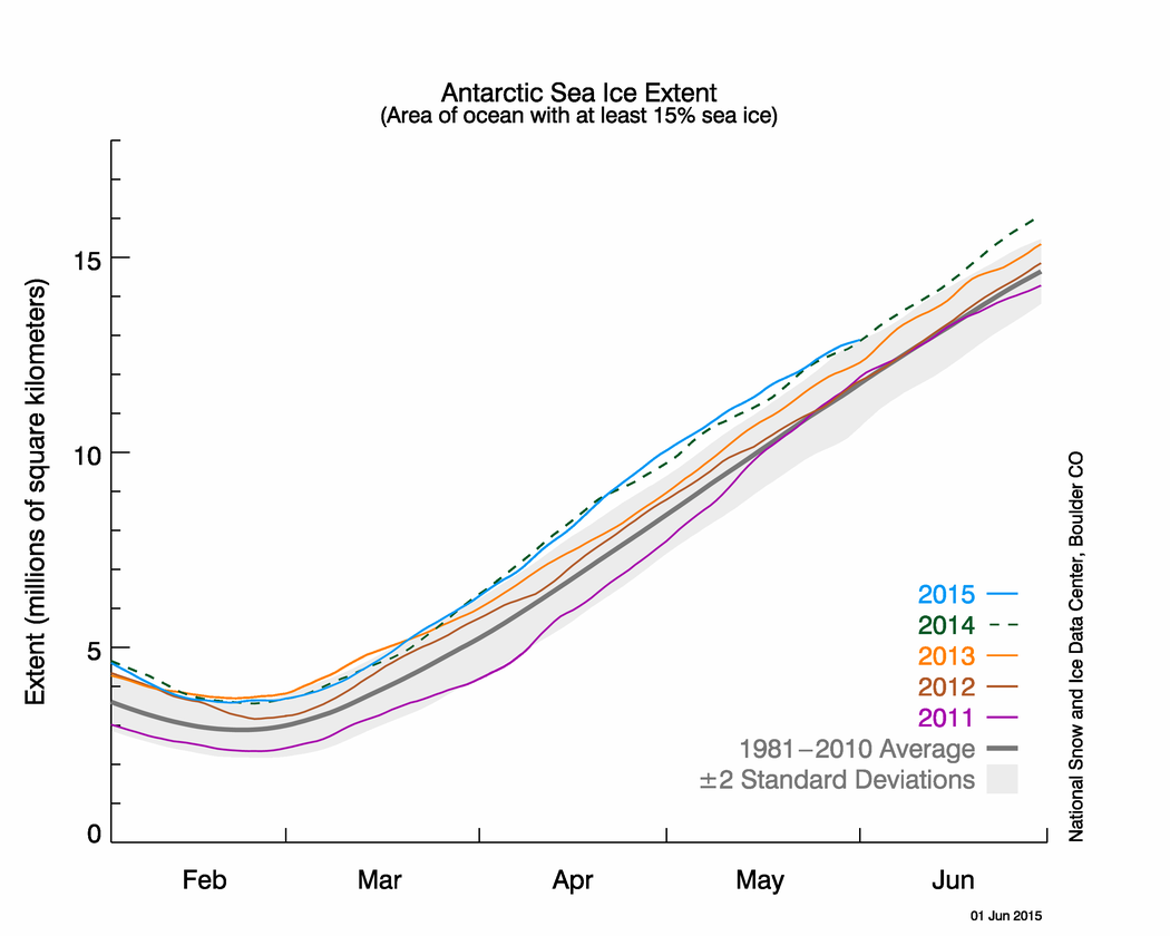
The rate of ice growth for the first half of November 2015 was quite rapid, but the pace of ice growth slowed during the second half of the month, only to increase again at the end of the month. Throughout the month, sea ice extent remained within two standard deviations of the 1981 to 2010 average.

Overview of conditions

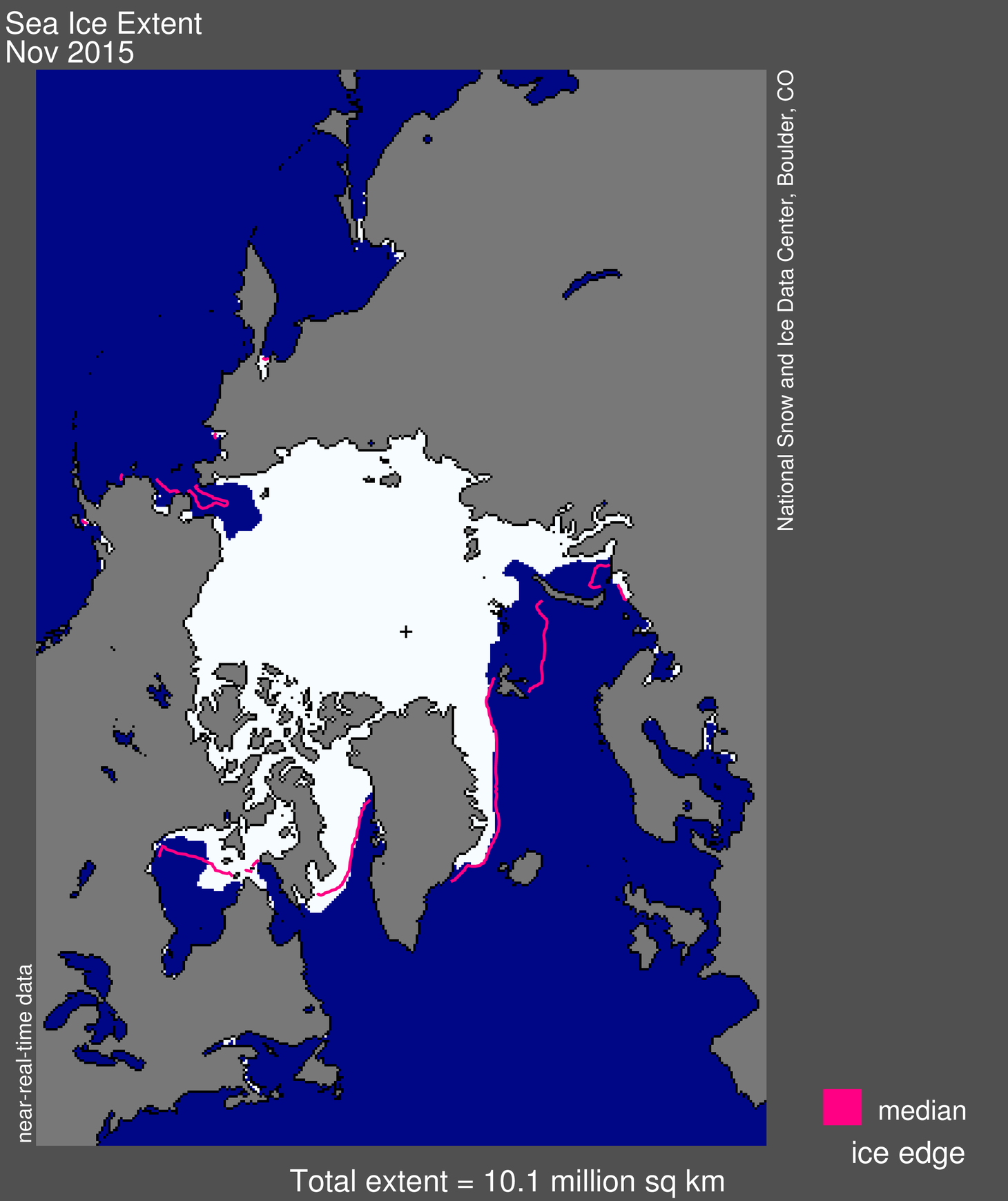
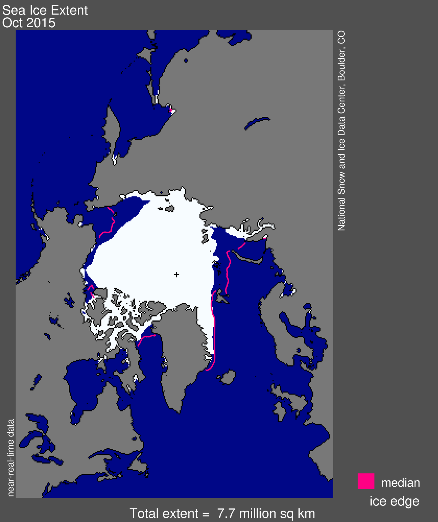
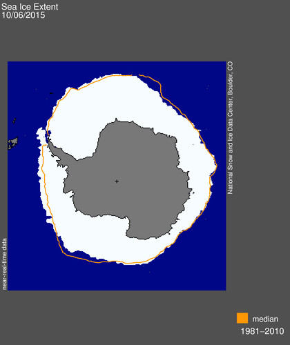
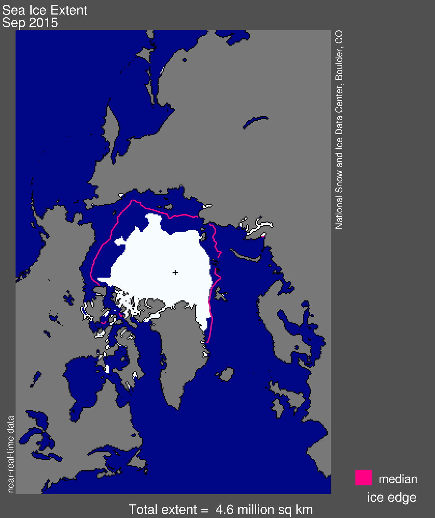
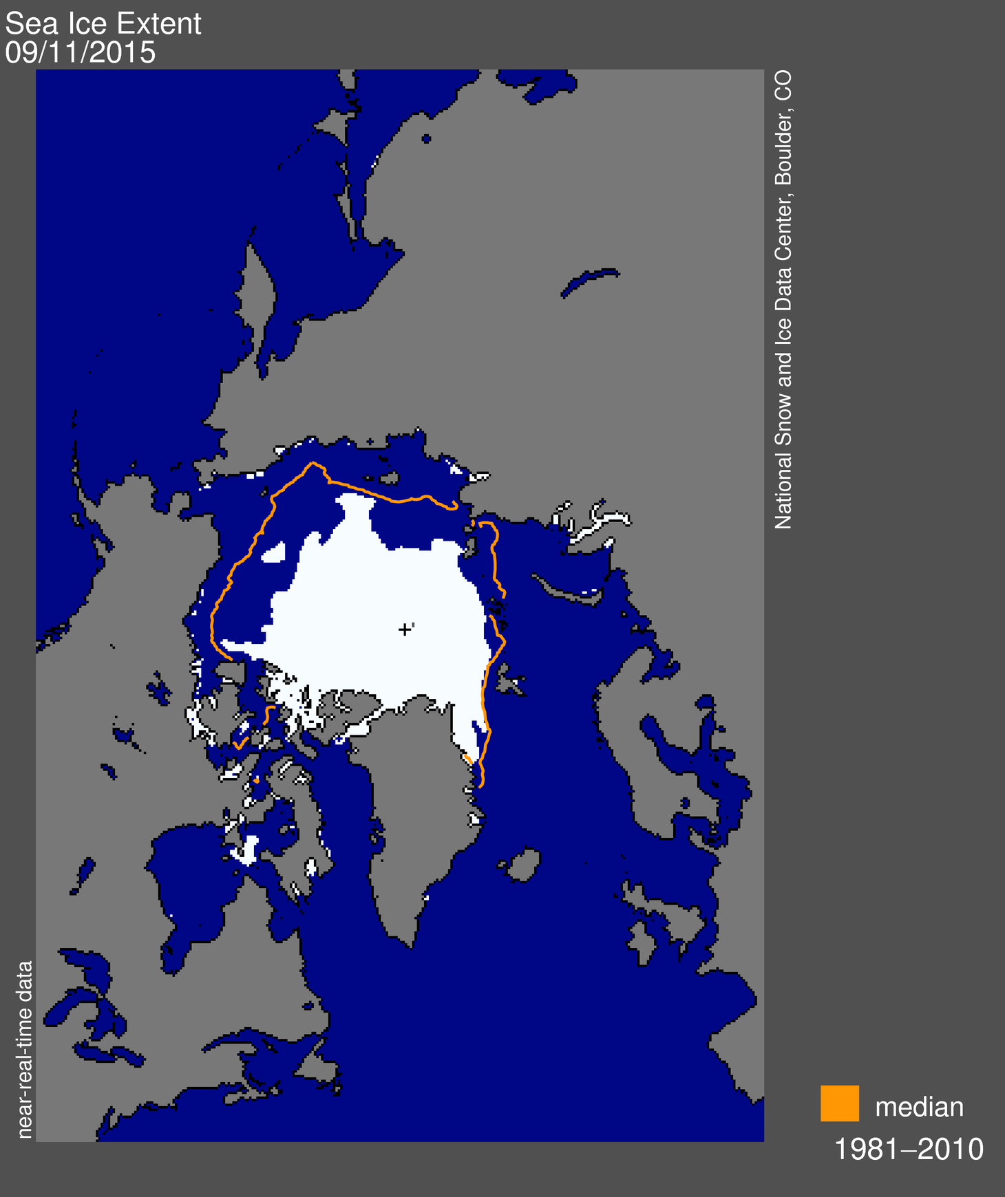
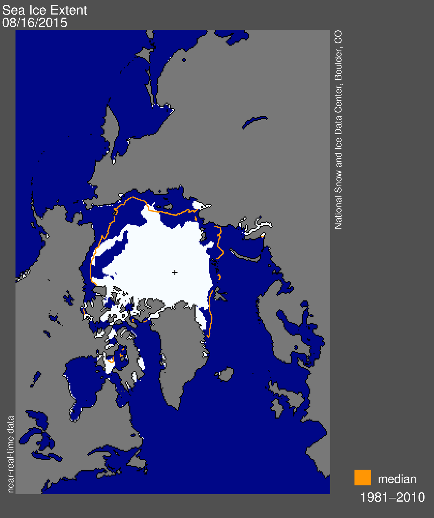
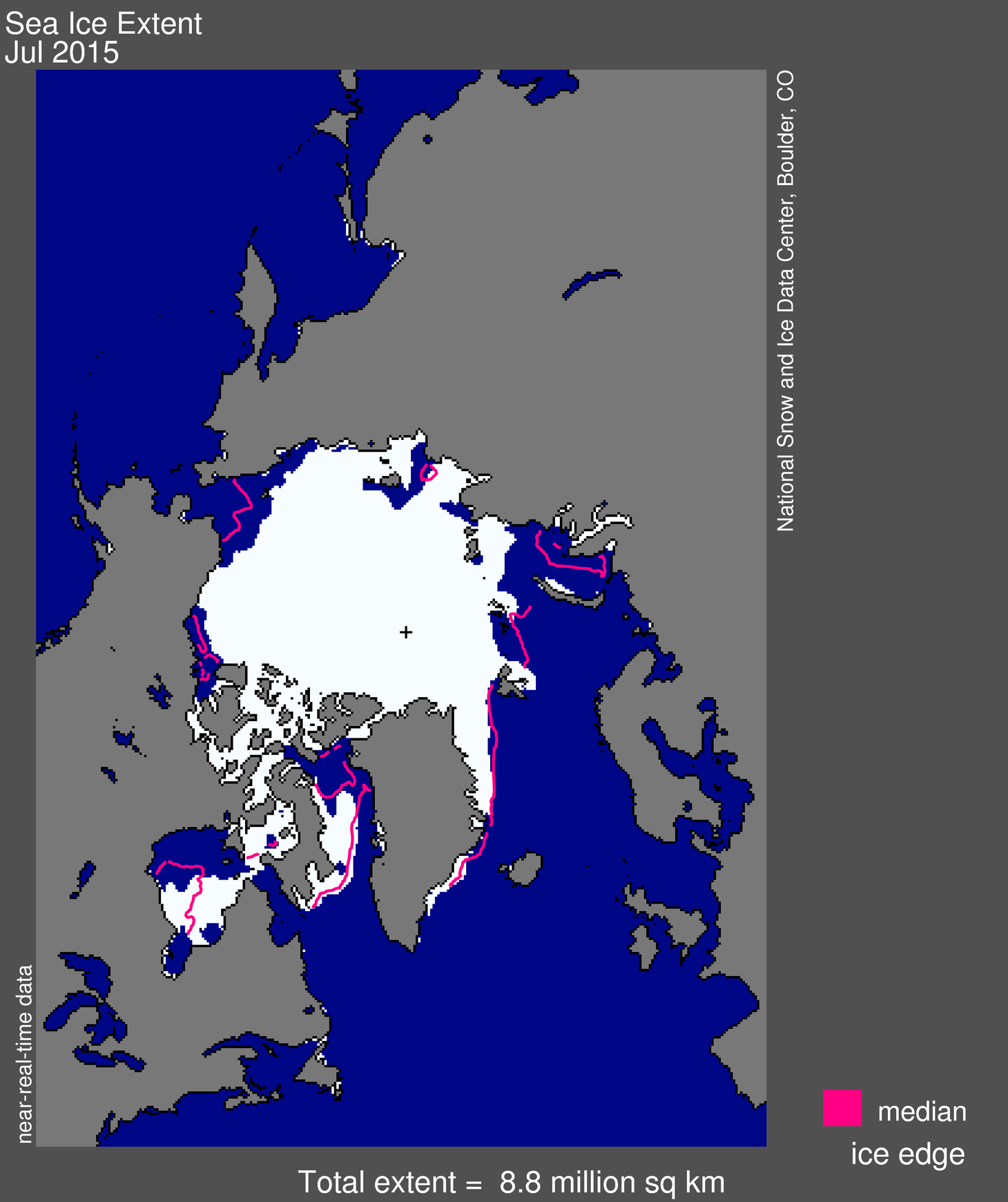
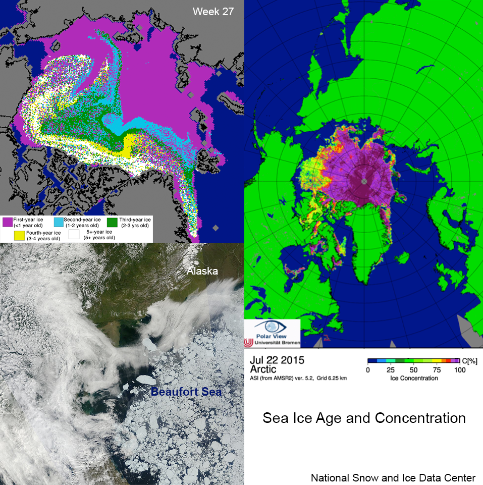
Figure 1. Arctic sea ice extent for November 2015 was 10.06 million square kilometers (3.88 million square miles). The magenta line shows the 1981 to 2010 median extent for that month. The black cross indicates the geographic North Pole. Sea Ice Index data. About the data

Credit: National Snow and Ice Data Center
High-resolution image

Arctic sea ice extent for November 2015 averaged 10.06 million square kilometers (3.88 million square miles), the sixth lowest November in the satellite record. This is 910,000 square kilometers (351,000 square miles) below the 1981 to 2010 average extent, and 230,000 square kilometers (89,000 square miles) above the record low monthly average for November that occurred in 2006. At the end of the month, extent was well below average in both the Barents Sea and the Bering Strait regions. Extent was above average in eastern Hudson Bay, but below average in the western part of the bay.

Conditions in context

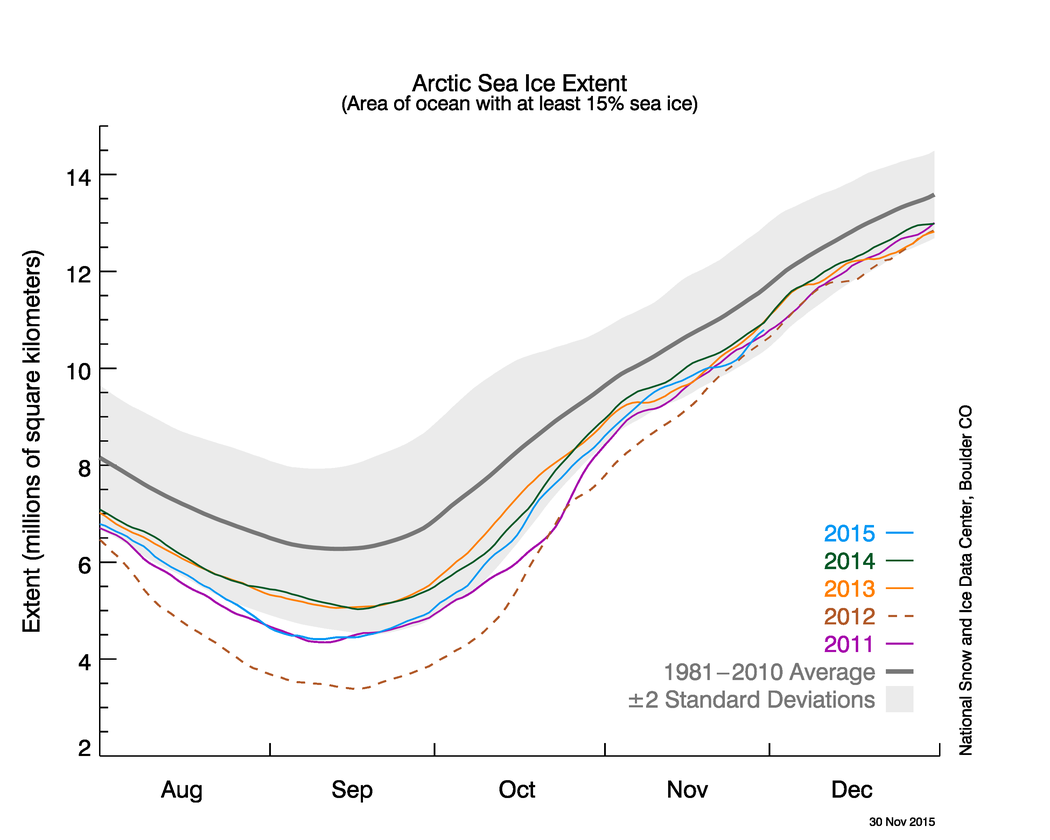
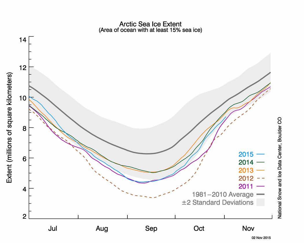
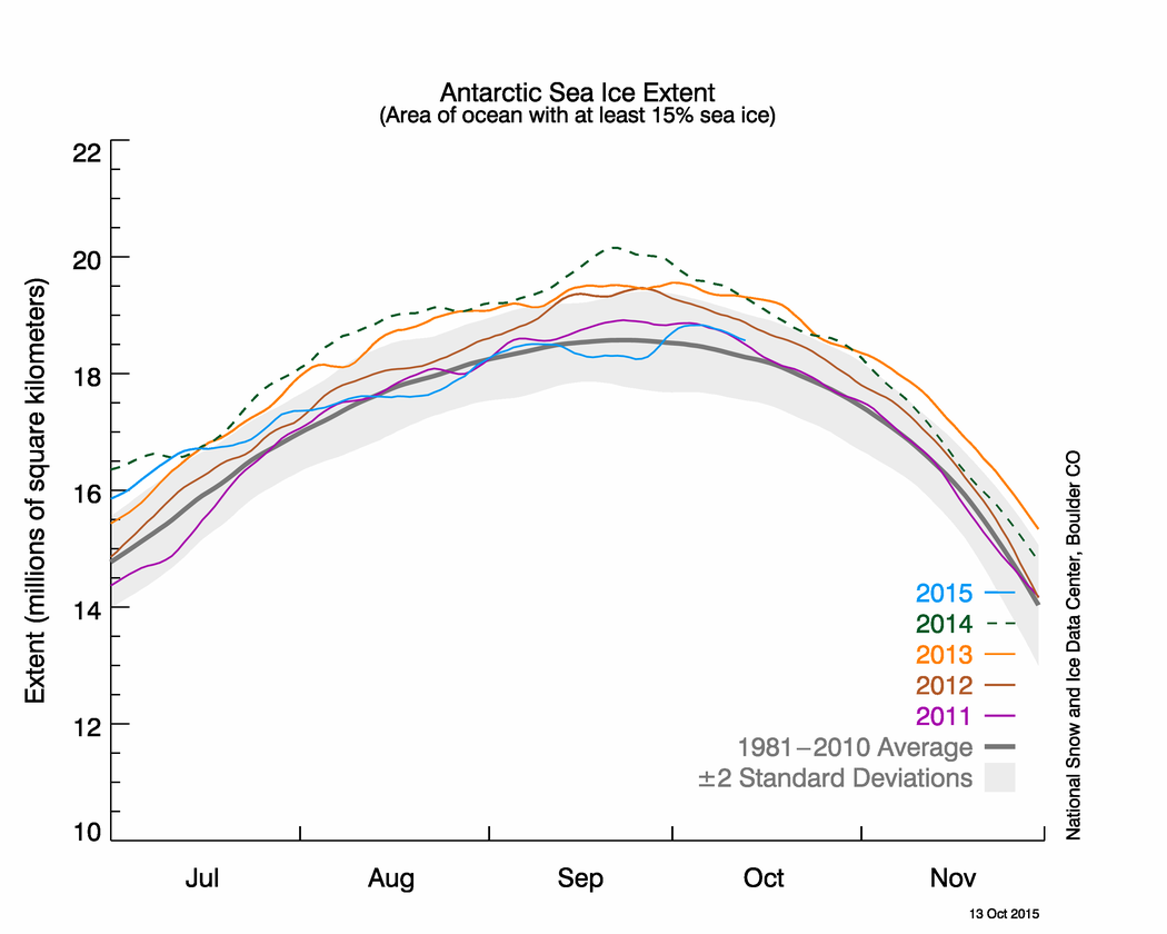
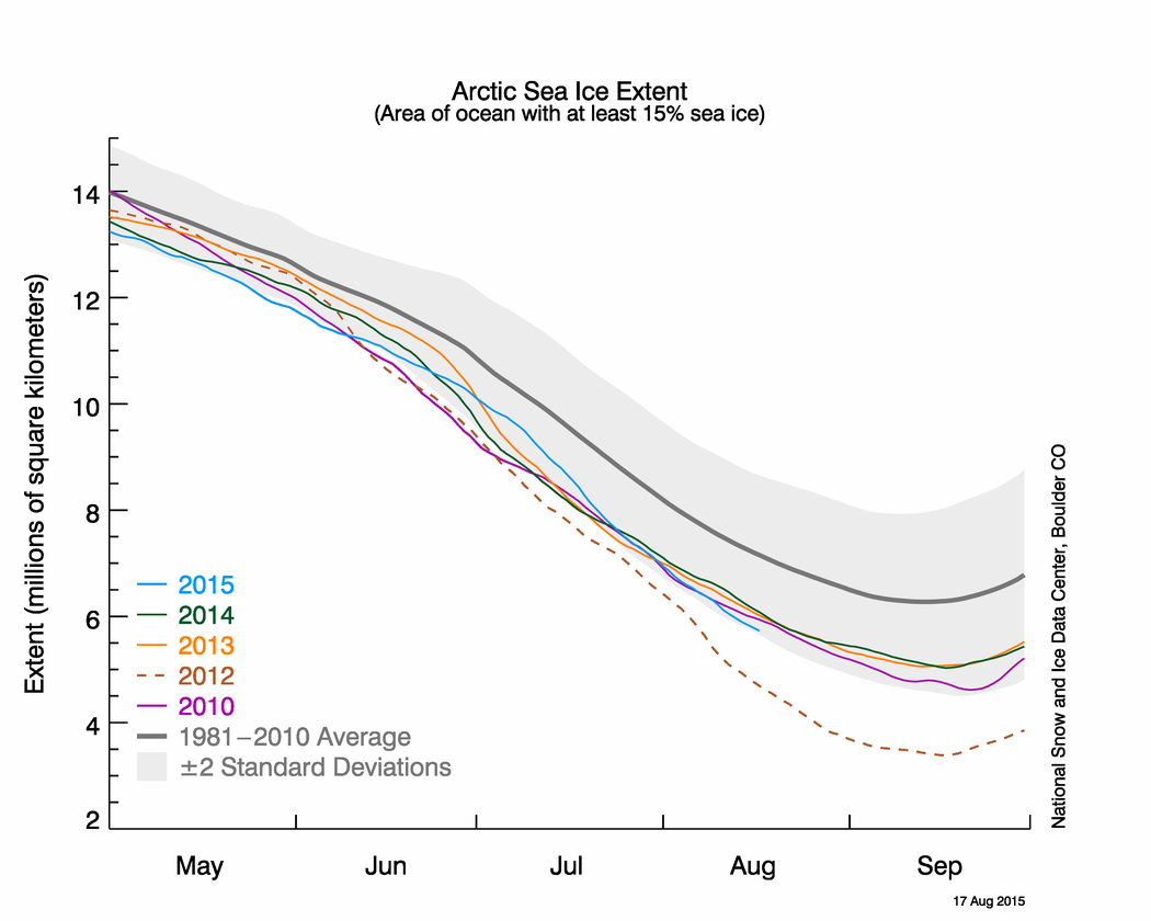
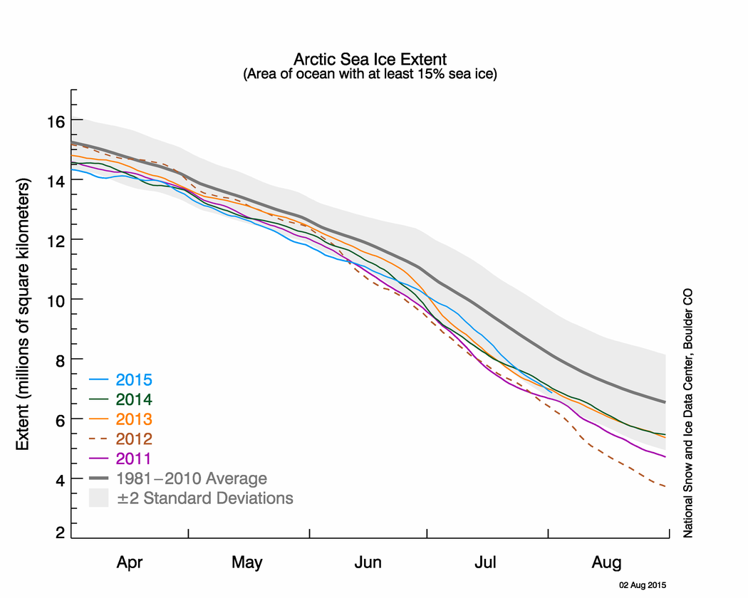
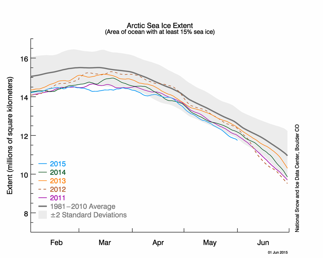
Figure 2a. The graph above shows Arctic sea ice extent as of November 30, 2015, along with daily ice extent data for four previous years. 2015 is shown in blue, 2014 in green, 2013 in orange, 2012 in brown, and 2011 in purple. The 1981 to 2010 average is in dark gray. The gray area around the average line shows the two standard deviation range of the data. Sea Ice Index data.

Credit: National Snow and Ice Data Center
High-resolution image

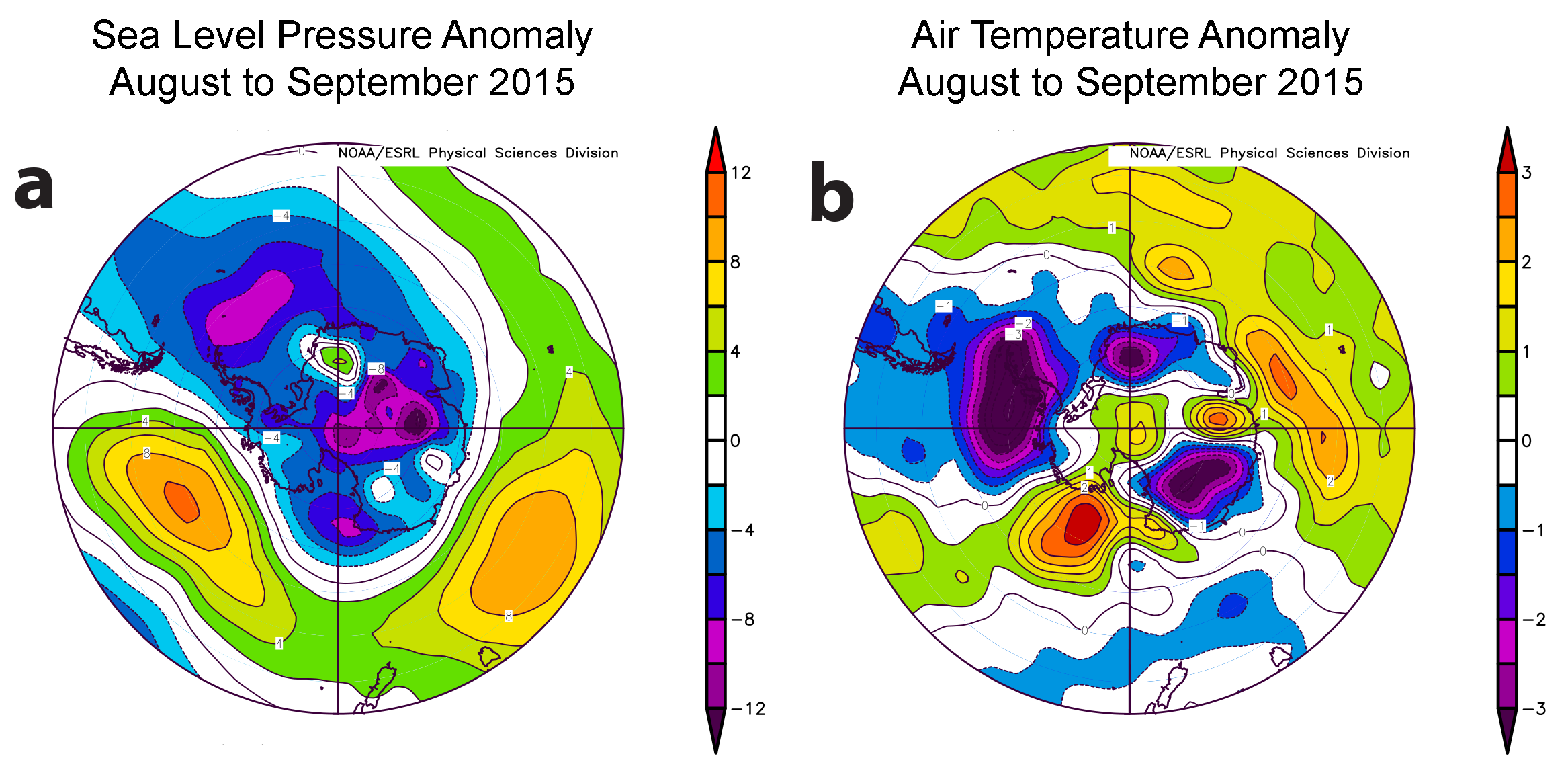
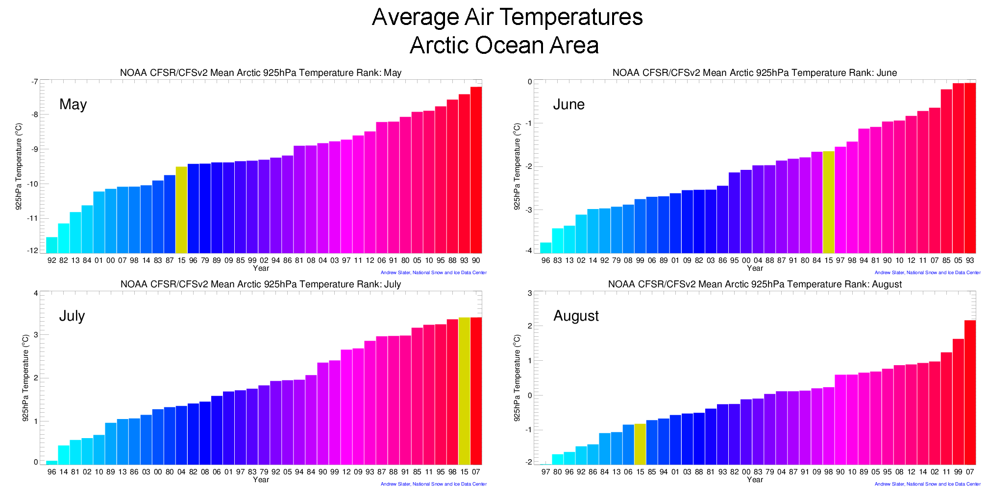
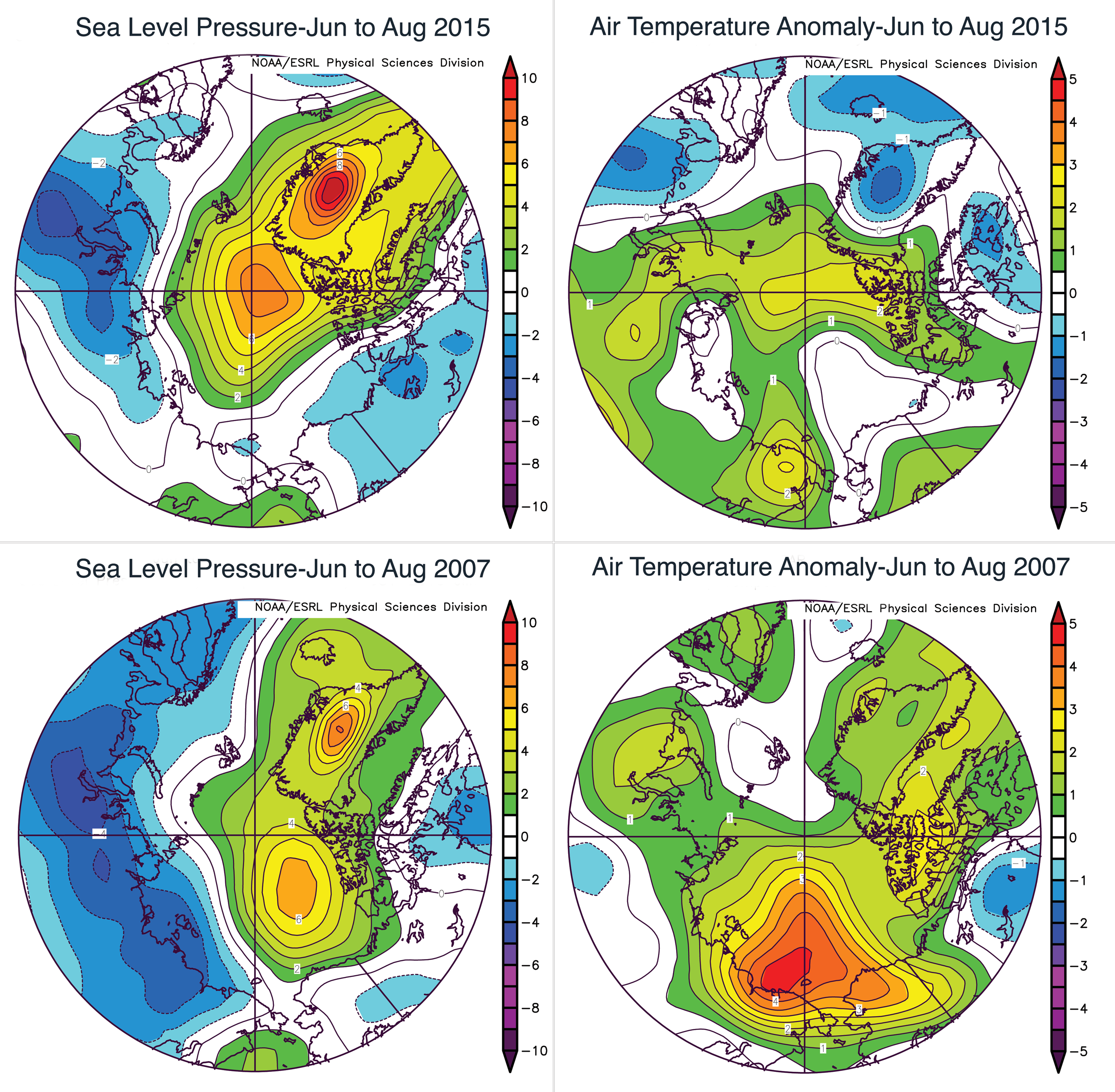
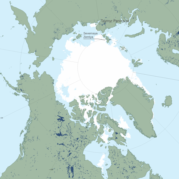
Air temperatures at the 925 millibar level were above average over nearly all of the Arctic Ocean; the area north of the Barents Sea, between Svalbard and the Taymyr Peninsula, was unusually warm (6 to 8 degrees Celsius, or 11 to 14 degrees Fahrenheit above average). Elsewhere, temperatures at the 925 millibar level were 1 to 4 degrees Celsius (2 to 7 degrees Fahrenheit) above average. NSIDC uses the 925 millibar temperature (about 3,000 feet above the surface) instead of the surface temperature because the 925 millibar temperature provides a better measure of overall warmth of the lower part of the atmosphere. From autumn through spring, the temperature at the surface can be greatly affected by the presence or absence of ice, while during summer, the surface temperature over ice will stay very close to the melting point.

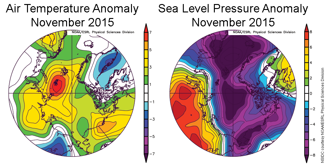
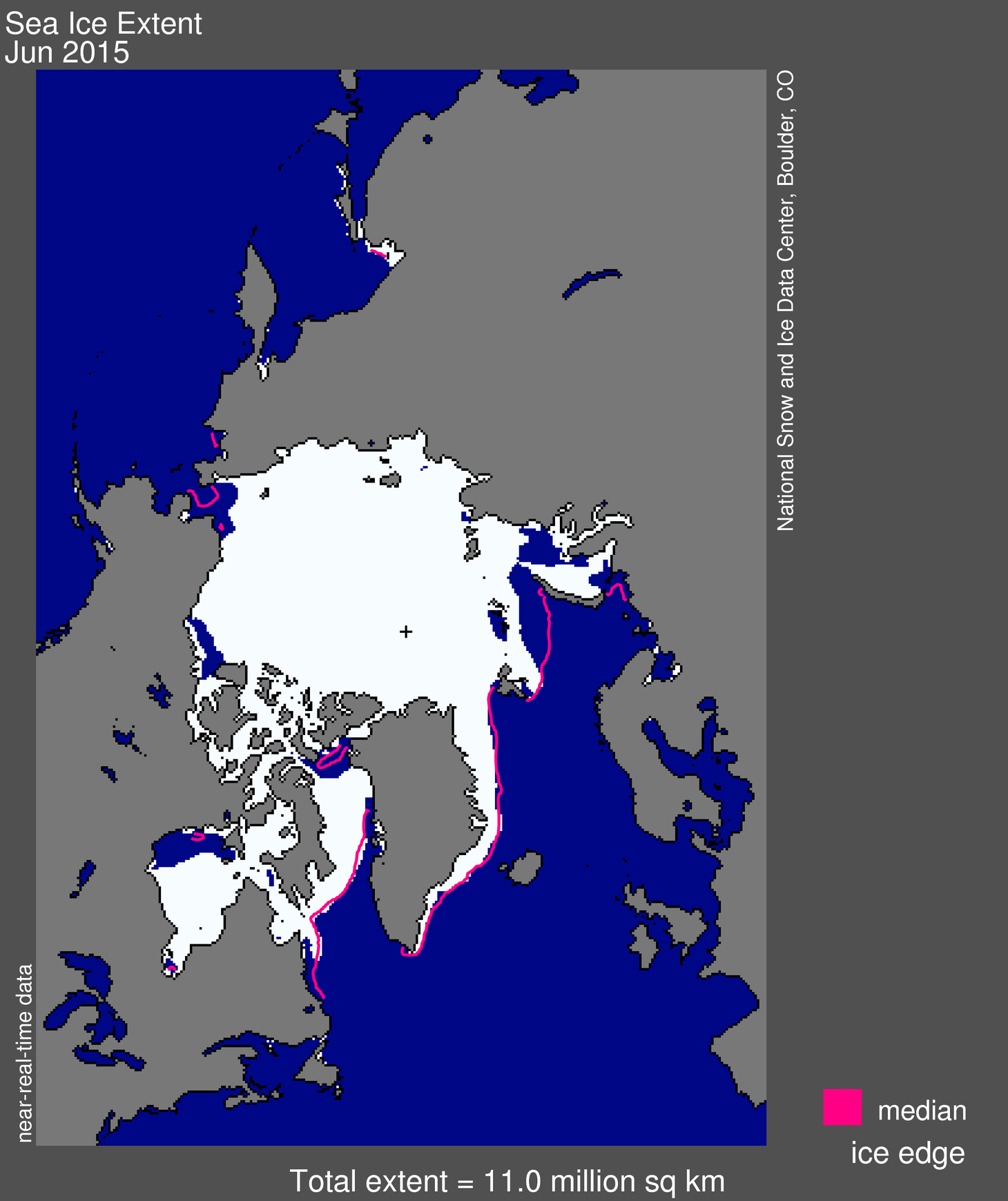
Figure 2b. The plot at left shows Arctic air temperature anomaly (difference from the 1981 to 2010 average) for November 2015 in degrees Celsius, at the 925 millibar level. Reds and yellows indicate higher than average temperatures for this month. The plot at right shows Arctic sea level pressure anomaly (difference from the 1981 to 2010 average) in millibars for November 2015. Sea level pressures were higher than average (red colors) over northern Eurasia, and lower than average (purples) over the Arctic Ocean and northern North Atlantic. This led to strong winds from the south and east over the region north of the Barents Seas, contributing to high temperatures in the area (observed at the 925 millibar level).

Credit: NSIDC courtesy NOAA/ESRL Physical Sciences Division
High-resolution image

The unusual warmth at the 925 millibar level north of the Barents Sea is related to an atmospheric circulation pattern featuring unusually high sea level pressure centered over northern Eurasia and unusually low pressure centered over the Arctic Ocean and northern North Atlantic. The strong pressure gradient (difference in pressure) between the areas of high and low pressure led to strong (and apparently warm) winds from the south. Open water in this area also extends unusually far to the north; while this likely contributed to above average temperatures even as high as the 925 millibar level, the wind pattern itself likely also helped to keep the ice from advancing south.

November 2015 compared to previous years

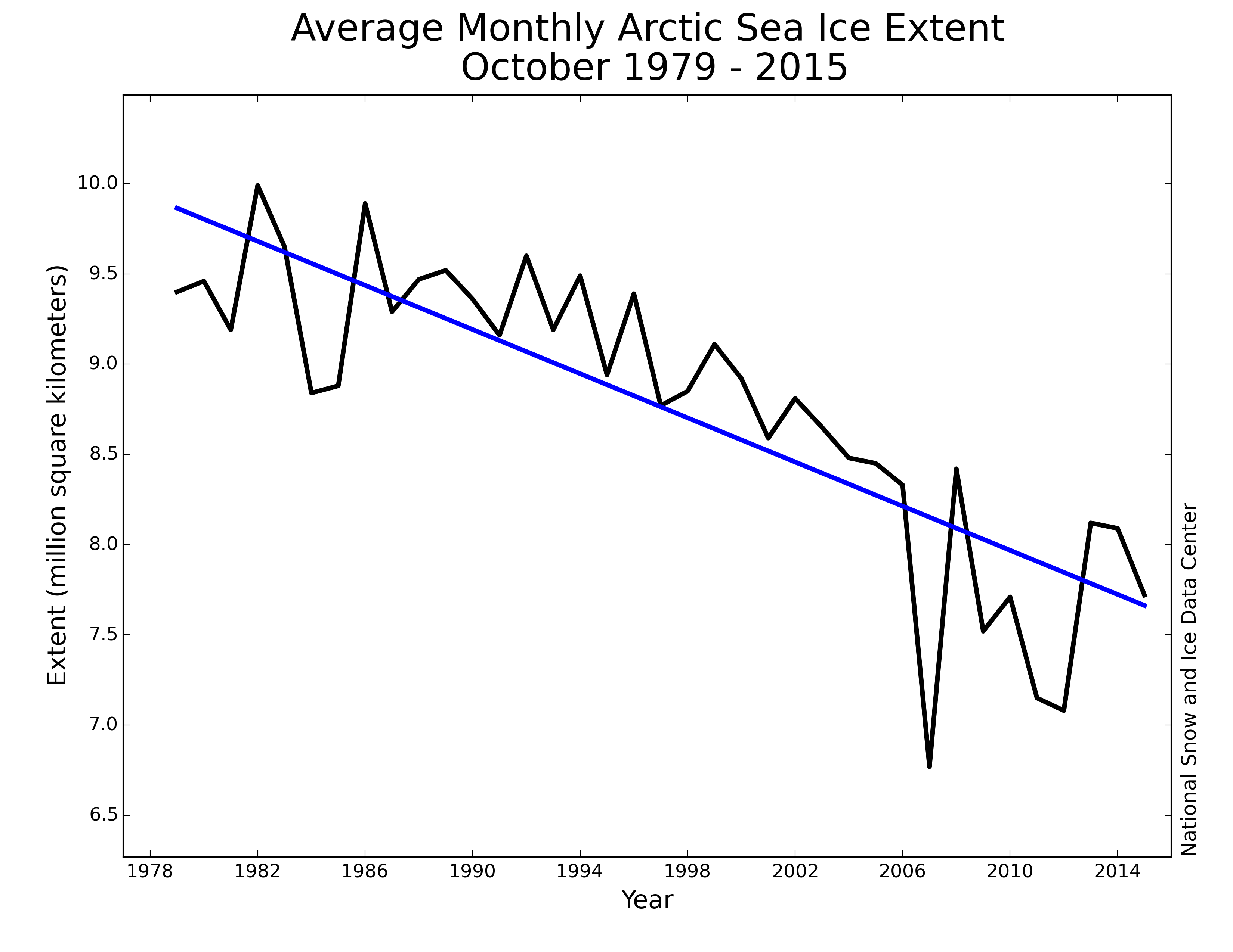
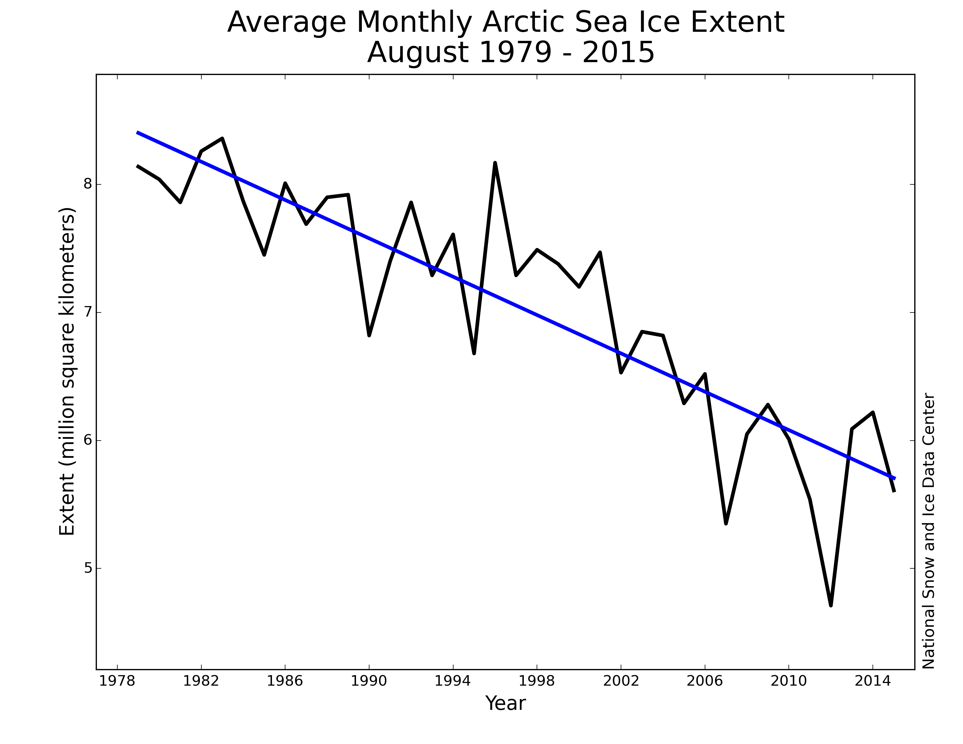
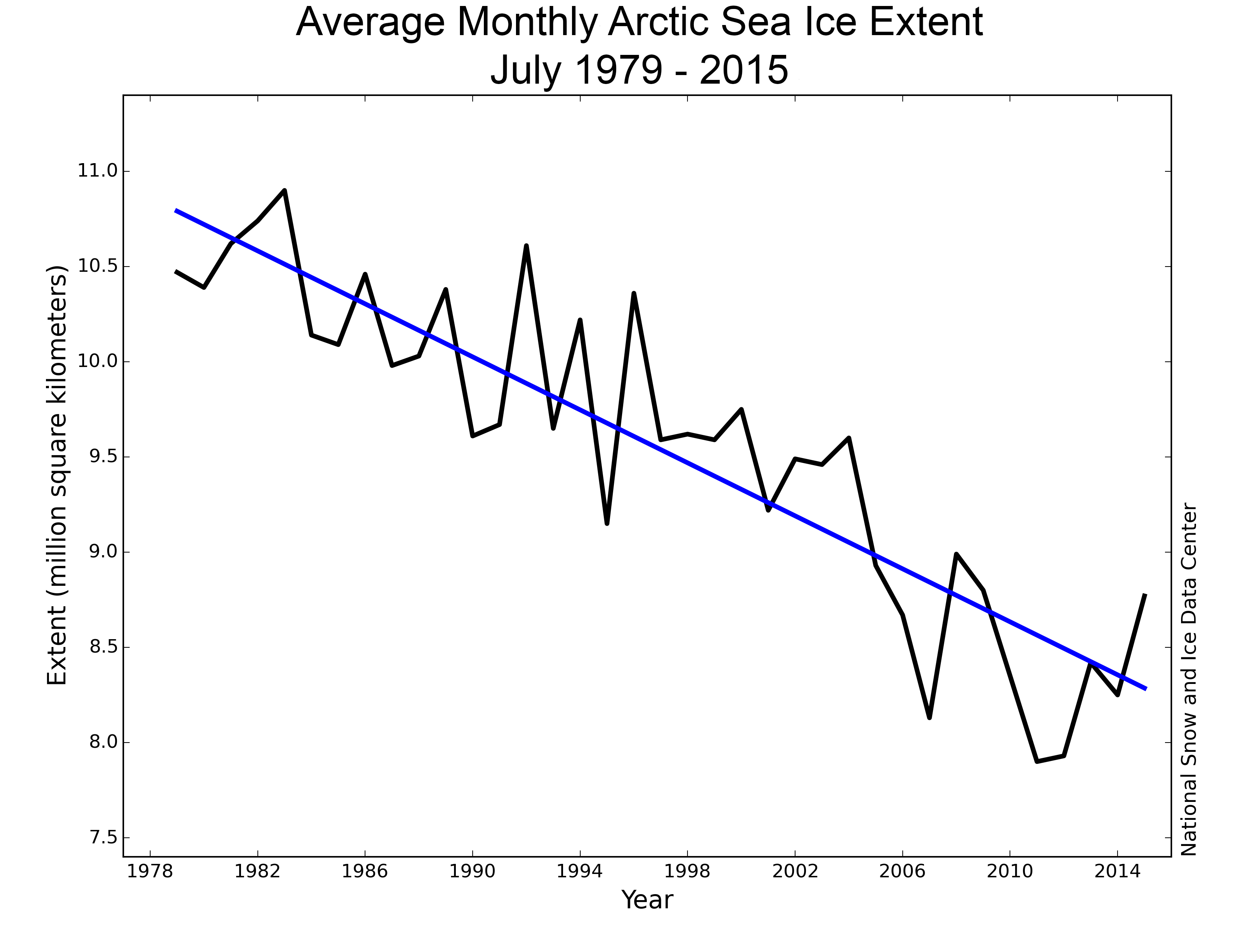
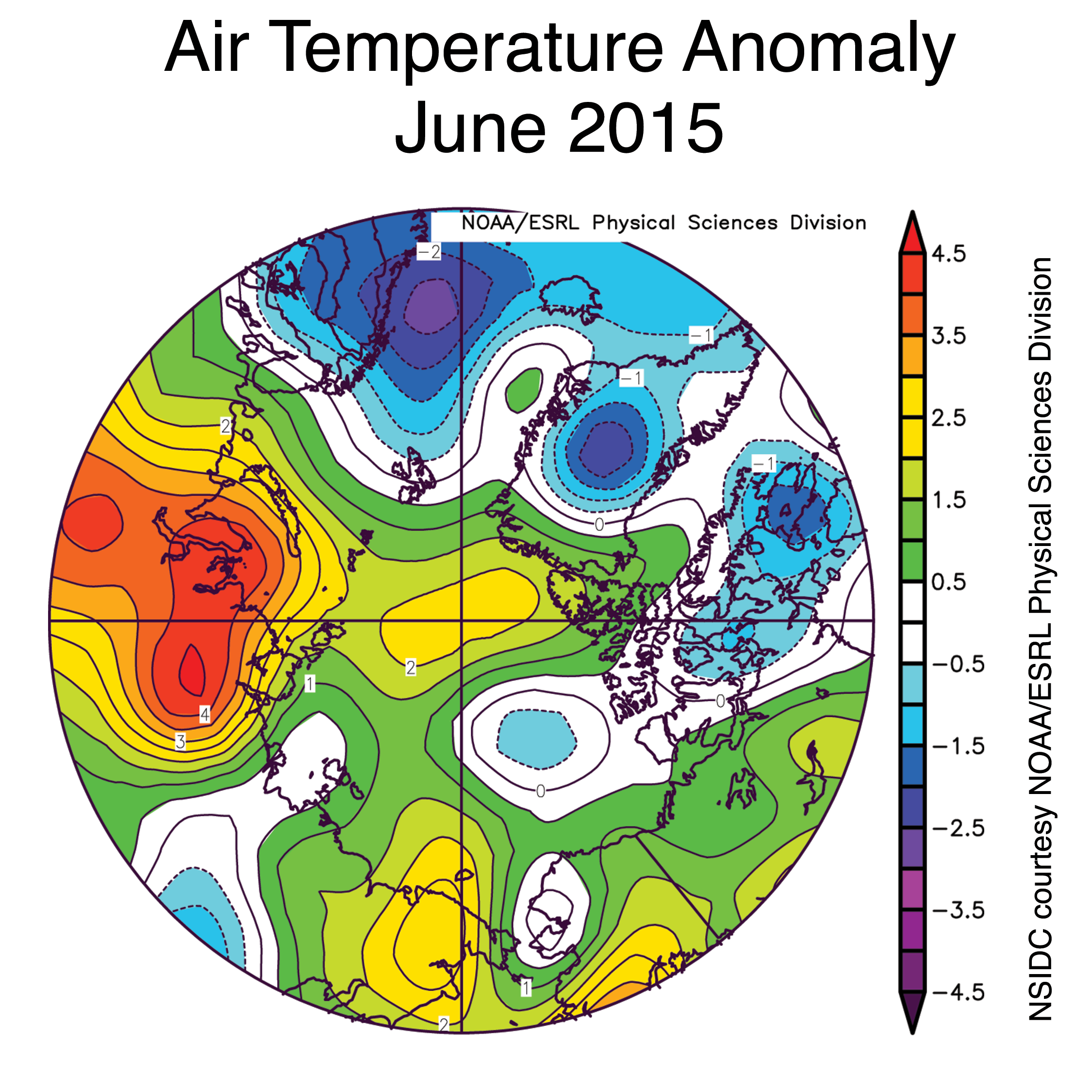
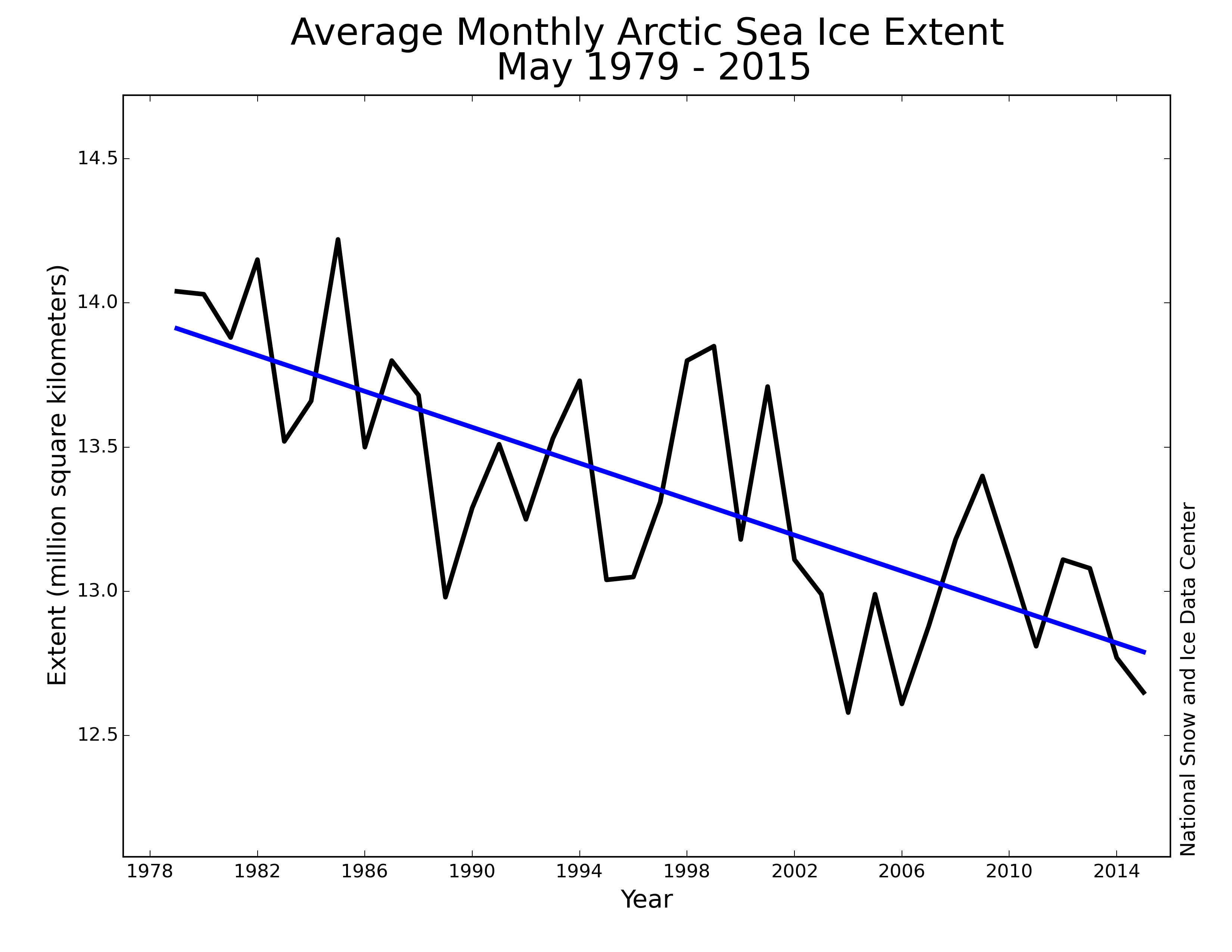
Figure 3. Monthly November ice extent for 1979 to 2015 shows a decline of 4.7% per decade.

Credit: National Snow and Ice Data Center
High-resolution image

Arctic sea ice extent averaged for November 2015 was the sixth lowest in the satellite data record. Through 2015, the linear rate of decline for November extent is 4.7% per decade.

The average rate of ice growth for November 2015 was 29,800 square kilometers per day (11,500 square miles per day). However, this value averages out the rather rapid growth rate during the first half of the month with a much slower rate during the second part of the month and rapid growth near its end.

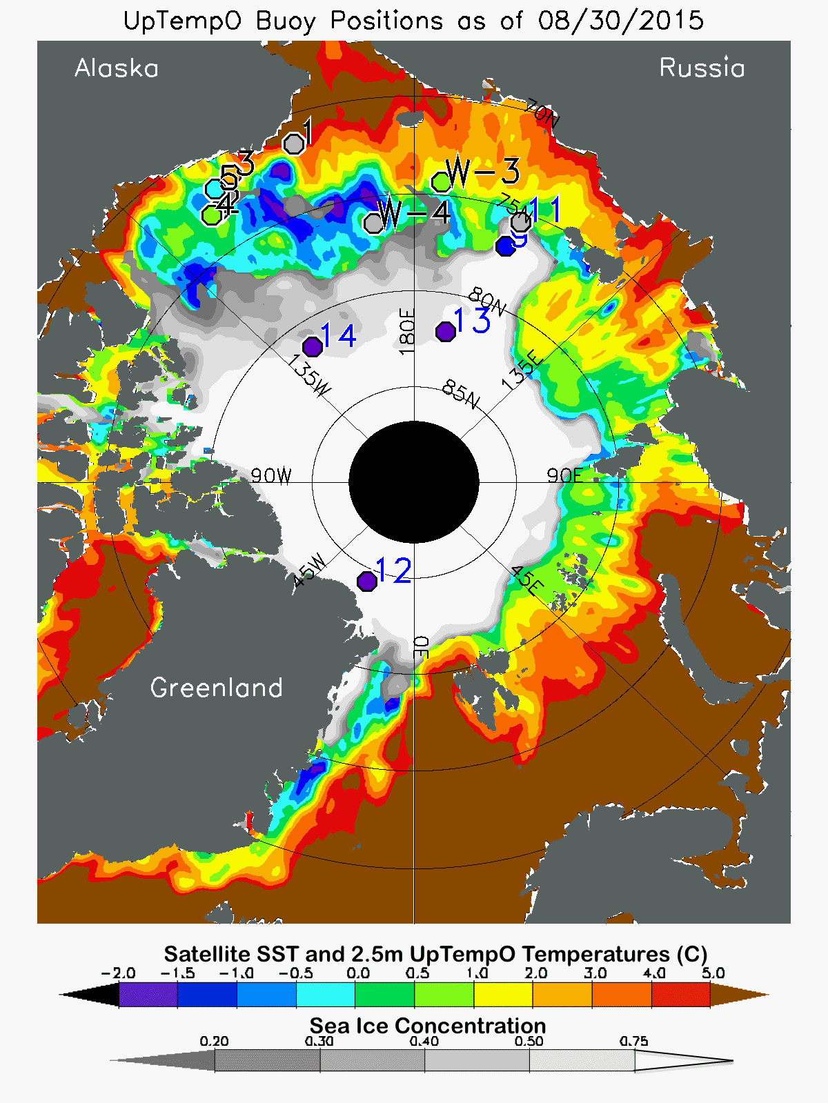
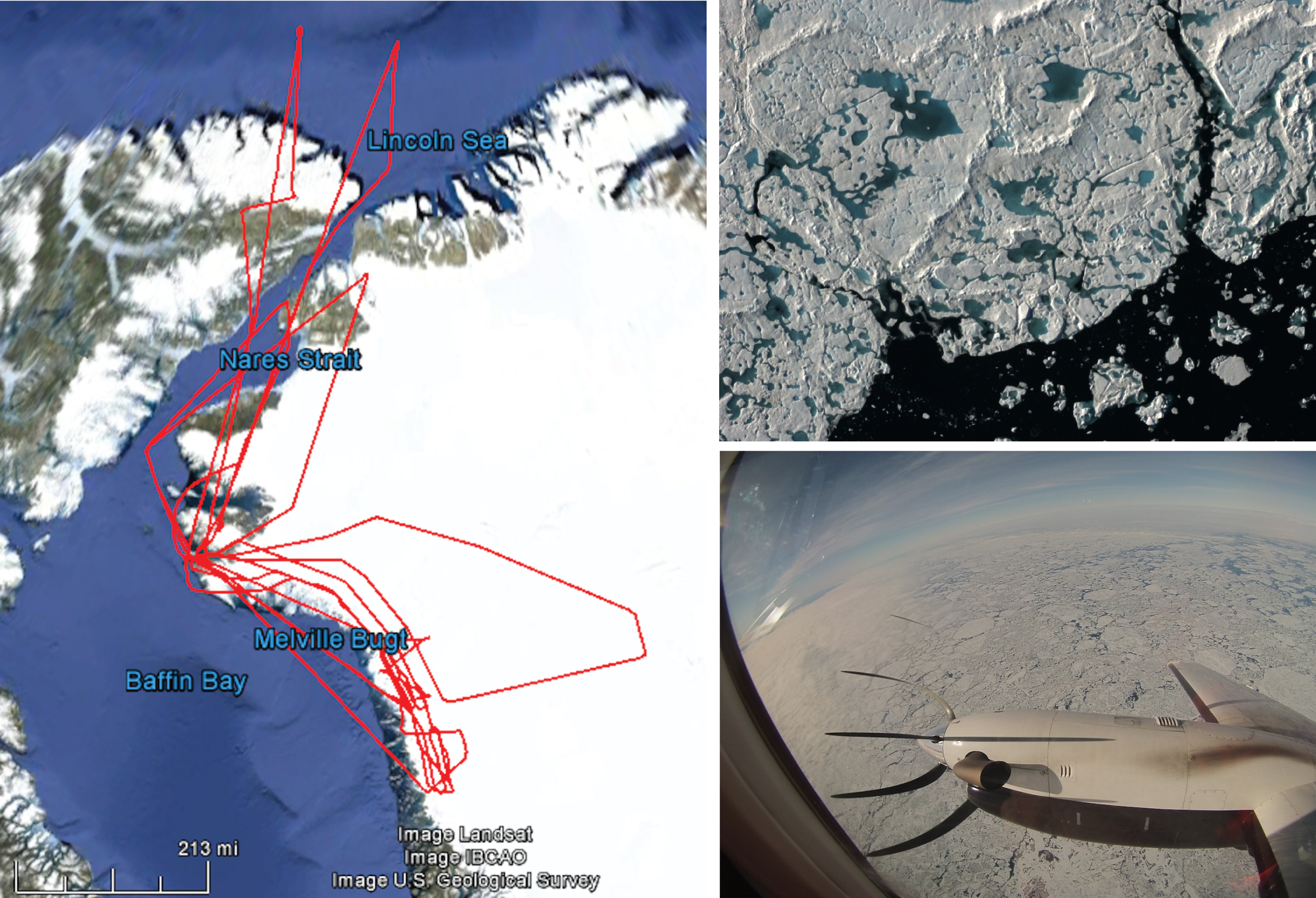
Loitering of the retreating sea ice edge in the Arctic seas

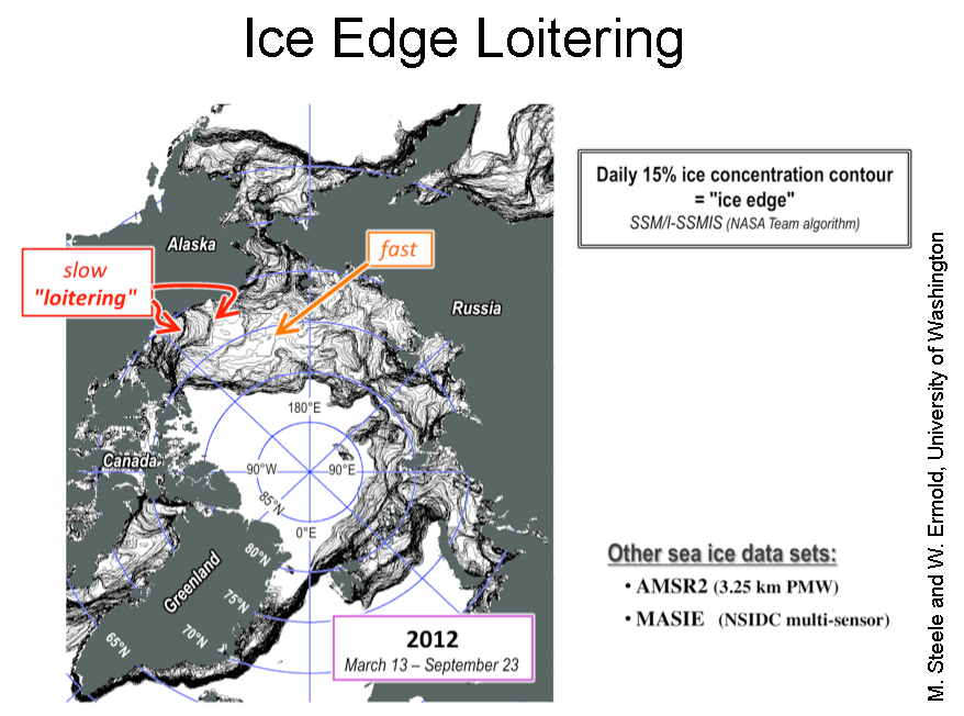
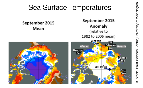
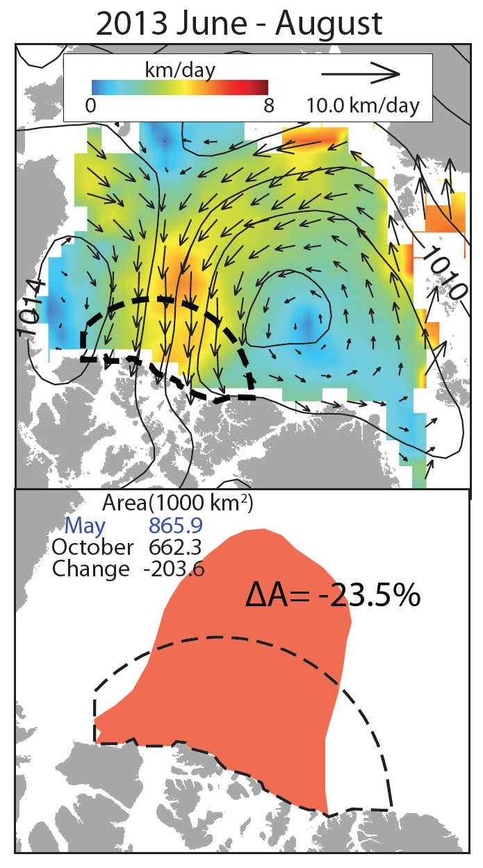
Figure 4. This image shows the daily average ice edge (thin black contours) for every day from March 13 to September 23, 2012. Constant ice edge retreat would produce equidistant contours through the retreat season. Instead, the contours point to areas of rapid retreat (where the contours are far apart, e.g., the central Amerasian Basin) and other areas where the ice edge retreat has stalled, or “loitered” (where the contours are over-plotting on top of themselves, producing darker areas, e.g., the Beaufort Sea). Some areas are prone to loitering in most years (north Baffin Bay; the east Beaufort, north Chukchi, Laptev, and Barents seas) and others are unlikely to see loitering behavior (west Beaufort, east Siberian seas).

Credit: M. Steele and W. Ermold, University of Washington
High-resolution image

A recent paper by colleagues M. Steele and W. Ermold of the University of Washington, in press with Journal of Geophysical Research Oceans, provides insight into pauses that are often observed in summer sea ice retreat. On some days, the ice in a region is observed to retreat at a rapid pace, while on others it hardly moves at all. Steele and Ermold term this stationary behavior “ice edge loitering.” They find that loitering occurs through interaction between surface winds and warm sea surface temperatures in areas from which the ice has already retreated. When ice retreat in a particular region happens early enough in the melt season, the water warms above the freezing point from being in contact with warmer and and from sunshine. If winds later in the season push the ice floes into the warmed ocean area, the ice floes will melt until that surface layer reaches the freezing point. Thus while individual ice floes are moving, the ice edge as a whole appears to remain fairly stationary. The time scale of loitering (typically, 4 to 7 days) is naturally tied to the typical time scale of passing weather systems.

Steele and Ermold argue that loitering likely has important effects on both physical and biological conditions at the ice edge during the summer. Consider an ice edge that retreats at a constant rate through the spring and summer. In this case, air/ice/ocean conditions remain fairly constant along the ice edge, simply translating northward with the ice edge through the summer. By comparison, loitering induces persistent melting and thus changes in sea ice morphology, enhances ocean stratification, reduces upwelling of nutrients, and leads to changes in the atmospheric boundary layer. If the wind then shifts and allows rapid northward ice retreat, what happens to the area of loitering that has been left behind? And what are the conditions within the rapidly retreating ice edge? These are questions for future studies.

Comparisons between observed and modeled September sea ice extent

Figure 4. This figure shows projected and hindcasted September sea ice extent (colors and shading) for climate models participating in the Intergovernmental Panel on Climate Change 5th Assessment, along with observations (black line). The projections are for four scenarios of greenhouse gas concentrations for the future (starting in 2006), termed Representative Concentration Pathways (RCPs) that relate to the radiative forcing at the top of the atmosphere that could occur at the year 2100. The shading indicates the one standard deviation range in the hindcasts and projections.

Credit: J. Stroeve and A. Barrett, National Snow and Ice Data Center
High-resolution image

A paper accepted for publication by NSIDC scientist Stroeve and colleagues includes model hindcasts and projections of September sea ice extent and comparisons with observed extent. The hindcasts and projections are from the global climate models that participated in the Intergovernmental Panel on Climate Change 5^th Assessment, and the observations include data that extend the record back to 1953.

The extent projections are shown for four different scenarios of future greenhouse gas growth (starting in 2005), termed Representative Concentration Pathways (RCPs). The RCPS relate to the radiative forcing at the top of the atmosphere that could occur at the year 2100. RCP 8.5 assumes a vigorous increase in greenhouse gas concentrations, while RCP 2.6 assumes a modest initial growth, followed by a reduction in concentrations. The shaded areas indicate the one standard deviation range of the sea ice extents projected by each model and the hindcasts.

The figure indicates that at least for the next few decades, which greenhouse gas scenario that becomes our reality is not especially important (there is much overlap between the projections). Instead, the simulated sea ice evolution is more strongly determined by both the natural variability in Arctic climate and by ongoing forcing from the current greenhouse gas content of the atmosphere. Only in the middle and later part of the 21^st century do the differences in the greenhouse gas concentration from the different scenarios become important, and even then, there is a large range in projections from the different models for the same RCP. If our future climate and greenhouse forcing follows RCP 2.6, September ice extent may begin to stabilize by around the middle of the century. Figures like this are useful to policy makers negotiating climate treaties at the Paris 2015 U.N. Climate Change Conference.

References

Steele, M. and W. Ermold. 2015. Loitering of the retreating sea ice edge in the Arctic Seas. J. Geophys. Res. Oceans, in press. doi:10.1002/2015JC011182.

Stroeve, J. and D. Notz. 2015. Insights on past and future sea-ice evolution from combining observations and models. Global and Planetary Change, in press. doi:10.1016/j.gloplacha.2015.10.011.

While Arctic sea ice extent is increasing, total ice extent remains below average, tracking almost two standard deviations below the long-term average.

Overview of conditions

Figure 1. Arctic sea ice extent for October 2015 was 7.72 million square kilometers (2.98 million square miles). The magenta line shows the 1981 to 2010 median extent for that month. The black cross indicates the geographic North Pole. Sea Ice Index data. About the data

Credit: National Snow and Ice Data Center
High-resolution image

Arctic sea ice extent for October 2015 averaged 7.72 million square kilometers (2.98 million square miles), the sixth lowest October in the satellite record. This is 1.19 million square kilometers (460,000 square miles) below the 1981 to 2010 average extent, and 950,000 square kilometers (367,000 square miles) above the record low monthly average for October that occurred in 2007.

Conditions in context

Figure 2. The graph above shows Arctic sea ice extent as of November 2, 2015, along with daily ice extent data for four previous years. 2015 is shown in blue, 2014 in green, 2013 in orange, 2012 in brown, and 2011 in purple. The 1981 to 2010 average is in dark gray. The gray area around the average line shows the two standard deviation range of the data. Sea Ice Index data.

Credit: National Snow and Ice Data Center
High-resolution image

Air temperatures at the 925 millibar level were 4 to 5 degrees Celsius (7 to 9 degrees Fahrenheit) above average over the central Arctic, extending towards Fram Strait. This appears to be due to unusually low pressure over northwest Greenland and higher pressures over the Tamyr Peninsula and Scandinavia, which funneled warm air from the south into the central Arctic Ocean. Coastal regions were generally 1 to 3 degrees Celsius (2 to 5 degrees Fahrenheit) higher than average.

October 2015 compared to previous years

Figure 3. Monthly October ice extent for 1979 to 2015 shows a decline of 6.9% per decade.

Credit: National Snow and Ice Data Center
High-resolution image

Through 2015, the October sea ice extent has declined 6.9% per decade over the satellite record.

New sea ice thickness information back for the winter

Figure 4a. This image from CryoSat-2 shows thin ice (less than 1 meter, or 3 feet, thick) over a wide area north of Greenland.

Credit: Center for Polar Observation and Modeling (CPOM) at University College London
High-resolution image

Figure 4b. This image from the European Space Agency’s Soil Moisture and Ocean Salinity (SMOS) satellite shows sea ice thickness over the Arctic Ocean.

Credit: University of Hamburg Integrated Climate Data Center
High-resolution image

In recent years, two European Space Agency (ESA) satellites, CryoSat-2 and SMOS (Soil Moisture and Ocean Salinity), have been providing information on sea ice thickness. Thickness information is valuable for assessing the overall condition of the sea ice cover. The sensors on these satellites cannot determine thickness during the summer melt season, but now that freeze-up has begun, information is again available.

CryoSat-2, launched in 2010, is a radar altimeter, which measures the height of the ice cover above the sea surface. Used with additional information on snow cover and its density, the height information can be converted into estimates of ice thickness. The Center for Polar Observation and Modeling (CPOM) at University College London has again started providing near-real-time maps of sea ice thickness from CryoSat-2.

While these maps are valuable in providing near-real-time thickness estimates, converting the satellite measurements into thickness involves complex processing and there are many uncertainties. For example, Figure 4a depicts thin ice (less than 1 meter [3 feet]) over a wide area north of Greenland, an area where wind and ocean current patterns push the ice against the coast forming thick ridges and an extremely rough surface. This area has been shown by other studies to have some of the thickest sea ice in the Arctic, often exceeding 4 meters (13 feet). This ridging may have cause the difficulty in the current mapping.

CryoSat-2 also has difficulty retrieving thickness in very thin sea ice regions, resulting in no thickness values reported at the outer edge of the ice cover. SMOS is a microwave imaging radiometer that measures microwave brightness temperature at a range that is sensitive to thin ice (1.4 gigahertz). These data are also now available in near-real-time at the University of Hamburg Integrated Climate Data Center. SMOS cannot estimate thickness beyond 1 meter (3.28 feet) at most and often not beyond 0.5 meters (1.64 feet). While the map shows a wide region of 1 meter-thick ice, it is important to realize that this is just the maximum allowable value and in reality there is thicker ice over much of the region. However, SMOS provides valuable information on the coverage of thin ice during the winter ice growth season. Ideally, a blended CryoSat-2/SMOS product will provide more comprehensive information on thickness.

A large ozone hole over the Antarctic

Figure 5. The image above shows the ozone hole over Antarctica on October 2, 2015 when it had reached its largest single-day area for the year, spanning 28.2 million square kilometers (10.9 million square miles). Data are from the Ozone Monitoring Instrument (OMI) on the NASA Aura satellite and the Ozone Monitoring and Profiler Suite (OMPS) on the NASA-NOAA Suomi NPP satellite.

Credit: NASA Earth Observatory, Ozone Hole Watch
High-resolution image

While sea ice in Antarctica is near average, the ozone hole over the continent grew relatively large during the austral winter. This goes against the expected trend towards a smaller ozone hole since the use of chlorofluorocarbons (CFCs) was banned in 1996. The size of the hole in a given year depends on several factors, including temperatures in the high altitude stratosphere. Temperatures in the Antarctic stratosphere were low this year, aiding chemical processes that destroy ozone. For more information on this year’s ozone hole see this NASA Earth Observatory feature.

Antarctic sea ice appears to have reached its annual maximum extent on October 6. The maximum occurred relatively late compared to past years. In contrast to the past three years, the 2015 maximum did not set a new record high for the period of satellite observations, but was nevertheless slightly above the 1981 to 2010 average.

Overview of conditions

Figure 1. Antarctic sea ice extent for October 6, 2015 was 18.83 million square kilometers (7.24 million square miles). The orange line shows the 1981 to 2010 median extent for that day. The black cross indicates the geographic South Pole. Sea Ice Index data. About the data

Credit: National Snow and Ice Data Center
High-resolution image

Antarctic sea ice extent reached its likely maximum for the year, at 18.83 million square kilometers (7.24 million square miles) on October 6, 2015. This year’s maximum was the sixteenth highest in the 35-year record. It was 120,000 square kilometers (46,000 square miles) above the average maximum daily extent computed over the 1981 to 2010 period of 18.71 million square kilometers (7.19 million square miles), and 1.33 million square kilometers (514,000 square miles) below the record maximum set in 2014. The date of the maximum was quite late in comparison to the 35-year satellite record. Only one year, 2002, has had a later maximum (October 12).

At the date of the 2015 maximum, Antarctic sea ice extent was greater than average in the Antarctic Peninsula region, the Weddell Sea, and the Wilkes Land coast area; and below average in the Ross Sea and Indian Ocean sectors.

Conditions in context

Figure 2. The graph above shows Antarctic sea ice extent as of October 13, 2015, along with daily ice extent data for four previous years. 2015 is shown in blue, 2014 in green, 2014 in orange, 2012 in brown, and 2011 in purple. The 1981 to 2010 average is in dark gray. The gray area around the average line shows the two standard deviation range of the data. Sea Ice Index data.

Credit: National Snow and Ice Data Center
High-resolution image

Figure 3. Panel (a) shows sea level air pressure anomaly for the Southern Ocean region, August 1 to September 30, 2015. Panel (b) shows air temperature anomaly for the Southern Ocean region, August 1 to September 30, at the 925 millibar level (approximately 1,600 feet altitude).

Credit: NOAA ESRL Physical Sciences Division
High-resolution image

Figure 4. The images compare Antarctic sea ice concentration for Septembers during two strong El Niño events (2015, left; 1997, right) to 1981 to 2010 averages. Colors show percent difference from average sea ice concentration surrounding Antarctica. Oranges and reds indicate concentrations higher than average; greens and blues indicate concentrations lower than average.

Credit: National Snow and Ice Data Center
High-resolution image

As recently as July 12, Antarctic sea ice extent was at a record daily high extent for the satellite period of observations. For much of early 2015, Antarctic sea ice extent was either slightly above or slightly below the levels seen on the same date in 2014, the record high year. However, beginning in mid-July, the growth rate for Antarctic sea ice slowed significantly, causing the 2015 maximum extent to be only the sixteenth highest in the record.

It is likely that this slowing of late-winter ice growth is related in part to the build-up of the El Niño conditions. El Niño occurs when a large area of the surface waters in the tropical eastern Pacific Ocean warms, and it has widespread effects on weather patterns. In the Southern Ocean, El Niño conditions are typically associated with a weakening of the Amundsen Sea Low, a persistent region of low air pressure in the southernmost Pacific sector of the Antarctic coast (Raphael et al., 2015). Air pressure in the Amundsen Sea region for the months of August and September was higher than average, indicating a weakening of the low-pressure tendency in the region. Higher-than-average air pressure was also observed in the Indian Ocean sector. These regions saw reduced sea ice growth and even local sea ice retreat as the austral winter progressed, and areas of higher-than-average temperatures near the ice edge.

Patterns of sea ice concentration around Antarctica (the deviation from average ice concentration) for El Niño years show a similar pattern, with more ice near the Peninsula.

References

Raphael, M. N., G. J. Marshall, J. Turner, R. Fogt, D. Schneider, D. A. Dixon, J. S. Hosking, J. M. Jones, and W. R. Hobbs. 2015. The Amundsen Sea Low: Variability, change and impact on Antarctic climate. Bulletin of the American Meteorological Society 2015, doi:10.1175/BAMS-D-14-00018.1.

The Arctic melt season has ended and sea ice extent is now increasing after reaching the fourth lowest minimum on record, on September 11. Sea ice extent in Antarctica has not yet reached its seasonal maximum.

Overview of conditions

Figure 1. Arctic sea ice extent for September 2015 was 4.63 million square kilometers (1.79 million square miles). The magenta line shows the 1981 to 2010 median extent for that month. The black cross indicates the geographic North Pole. Sea Ice Index data. About the data

Credit: National Snow and Ice Data Center
High-resolution image

Following the seasonal daily minimum of 4.41 million square kilometers (1.70 million square miles) that was set on September 11, which was the fourth lowest in the satellite record, Arctic sea ice has started its cycle of growth. Arctic sea ice extent averaged for the month of September 2015 was 4.63 million square kilometers (1.79 million square miles), also the fourth lowest in the satellite record. This is 1.87 million square kilometers (722,000 square miles) below the 1981 to 2010 average extent, and 1.01 million square kilometers (390,000 square miles) above the record low monthly average for September that occurred in 2012. As of this writing, Antarctica’s winter maximum has not yet occurred, but is anticipated within several days.

Conditions in context

Figure 2. The graph above shows Arctic sea ice extent as of October 5, 2015, along with daily ice extent data for four previous years. 2015 is shown in blue, 2014 in green, 2013 in orange, 2012 in brown, and 2011 in purple. The 1981 to 2010 average is in dark gray. The gray area around the average line shows the two standard deviation range of the data. Note: This graph was updated to show the most recent years, in order to be consistent with our monthly posts. Sea Ice Index data.

Credit: National Snow and Ice Data Center
High-resolution image

For two weeks following the minimum extent on September 11, air temperatures at the 925 hPa level (about 3,000 feet above the surface) were 2 to 4 degrees Celsius (4 to 7 degrees Fahrenheit) lower than average in the Chukchi and Beaufort seas, helping foster ice growth in those regions. Elsewhere over the Arctic Ocean, there has been fairly little ice growth, in part due to near average to slightly above average air temperatures. Both the Northern Sea Route and Roald Amundsen’s route through the Northwest Passage appeared to remain free of ice at the end of the month. The deeper northern route through Parry Channel, which consists of M’Clure Strait, Barrow Strait, and Lancaster Sound, never completely cleared of ice.

September 2015 compared to previous years

Figure 3. Monthly September ice extent for 1979 to 2015 shows a decline of 13.4% per decade relative to the 1981 to 2010 average.

Credit: National Snow and Ice Data Center
High-resolution image

Through 2015, the linear rate of decline for September Arctic ice extent over the satellite record is 13.4% per decade. The nine lowest September ice extents over the satellite record have all occurred in the last nine years.

Conditions leading to this year’s minimum

Figure 4a. The map at left shows multiyear ice fraction in mid-April derived from ASCAT, and the corresponding map at right shows ice age. ASCAT image courtesy of R. Kwok, NASA Jet Propulsion Laboratory. Ice age image derived from data provided by M. Tschudi, University of Colorado Boulder.

Credit: National Snow and Ice Data Center
High-resolution image

Figure 4b. The graphs show Arctic ocean air temperatures for May, June, July, and August at the 925 hPa level, ranked according to year from lowest (in blue colors) to highest (in red colors). Ranking of 2015 is given in yellow.

Credit: D. Slater, National Snow and Ice Data Center
High-resolution image

Figure 4c. The maps show Arctic sea surface temperature (SST) and anomaly in degrees Celsius, for September 2015. The image at left shows average temperature, with reds indicating higher temperatures and blues indicating lower temperatures. The map at right shows temperature anomaly, compared to the 1982 to 2006 average. Reds and oranges indicate higher than average temperatures, and blues lower than average. The grey line indicates the sea ice edge. SSTs are from from the NCDC OIv2 “Reynolds” data set, a blend of satellite (AVHRR) and in situ data designed to provide a “bulk” or “mixed layer” temperature. Ice edge is from NSIDC near real time passive microwave data.

Credit: M. Steele, Polar Science Center/University of Washington
High-resolution image

The summer melt season began earlier than average. The maximum winter extent, reached on February 25, 2015, was also the lowest recorded over the period of satellite observations. However, a relatively large amount of multiyear ice was transported into the southern Beaufort and Chukchi seas during the winter, as documented by images of multiyear ice fraction derived from the Advanced Scatterometer (ASCAT) instrument on the METOP-A satellite (Figure 4a). The corresponding ice age image shows that the multiyear ice largely consisted of floes that had survived several melt seasons, indicating that it was fairly thick. Thick ice is more difficult to melt out during summer than thinner ice; if not for this thicker ice, the September minimum extent would likely have been lower.

Melt onset began earlier than average in the Beaufort Sea, especially along the coast of Canada, leading to early development of open water in this area. Melt also began earlier than is usual in the Kara Sea, fostering early retreat of sea ice in the region. However, air temperatures at the 925 hPa level during May and June for the Arctic ocean region were not particularly high, ranking as the 26^th and 13^th warmest since 1979 (Figure 4b). As a result, although the winter maximum extent was the lowest in the satellite record, ice extent at the end of June was only the third lowest.

The pace of seasonal ice loss picked up rapidly in July, with Arctic ocean region temperatures at the 925 hPa level reaching the second highest during the satellite record (with 2007 ranked as the highest). Daily ice loss rates averaged 101,800 square kilometers (39,300 square miles) per day, the fourth largest rate of ice loss recorded for the month. Nevertheless, sea ice was slow to melt out of Baffin Bay and Hudson Bay, resulting in a July average extent for 2015 that was the eighth lowest on record. By the end of July however, the fast pace of ice loss during the month resulted in 2015 extent falling within 550,000 square kilometers (212,000 square miles) of the level recorded in 2012, and tracking below the levels recorded for 2013 and 2014. By the middle of August, the difference in extent between 2012 and 2015 had dropped to less than 500,000 square kilometers (193,000 square miles), hinting at the possibility that this year would rank among the lowest minimum extents recorded. However, temperatures for August were not particularly warm, and extent ended up fourth lowest.

Higher than average Arctic sea surface temperatures dominated the Arctic Ocean in September 2015 (Figure 4c), though not as high as seen in 2007 or 2012. Early melt onset as well as strong spring winds in the eastern Beaufort Sea led to early ice retreat in this area (Steele et al., 2015). These winds were particularly strong in April 2015, but then they abated, so that while the resulting summer sea surface temperatures were higher than surrounding waters, they were only around 2 to 3 degrees Celsius (4 to 5 degrees Fahrenheit) higher than average near the coast. The Kara Sea was also unusually warm this year, while sea surface temperatures were generally lower than average in the Nordic seas.

What happened to the old ice in the Beaufort and Chukchi Seas?

Figure 5a. The map shows Arctic sea ice age, in years, for the week of September 7 to 13, 2015.

Credit: M. Tschudi, University of Colorado Boulder
High-resolution image

Figure 5b. The plot shows survival rates of first-year, second-year, and older ice, in percentage of area that survived.

Credit: National Snow and Ice Data Center
High-resolution image

Maps of ice age at the beginning of the melt season and at the time of the September minimum extent (Figure 5a) reveal that most of the old ice transported into the southern Beaufort and Chukchi seas melted out this summer. This resulted in a 31% depletion of the multiyear ice cover this summer for the Arctic as a whole, compared to only 12% in 2013 and 38% in 2012. There was also more first-year ice lost this summer than during the last two summers. Sixty-two percent of the winter first-year ice was lost. Overall, this was the third largest amount of first-year ice lost in a melt season, behind 2012 (73%) and 2007 (67%).

References

Steele, M., S. Dickinson, J. Zhang, and R. Lindsay. 2015. Seasonal ice loss in the Beaufort Sea: Toward synchrony and prediction, J. Geophys. Res., 120, doi:10.1002/2014JC010247.

Erratum

A reader alerted us that Figure 5a was mislabeled. Instead of Mid-March 2015, it should have been labeled September 2015. On October 8, 2015, we corrected the label and its caption.

August saw a remarkably steady decline in Arctic sea ice extent, at a rate slightly faster than the long-term average. Forecasts show that this year’s minimum sea ice extent, which typically occurs in mid to late September, is likely to be the third or fourth lowest in the satellite record. All four of the lowest extents have occurred since 2007. In mid-August, Antarctic sea ice extent began to trend below the 1981 to 2010 average for the first time since November 2011.

Overview of conditions

Figure 1. Arctic sea ice extent for August 2015 was 5.61 million square kilometers (2.16 million square miles). The magenta line shows the 1981 to 2010 median extent for that month. The black cross indicates the geographic North Pole. Sea Ice Index data. About the data

Credit: National Snow and Ice Data Center
High-resolution image

Average sea ice extent for August 2015 was 5.61 million square kilometers (2.16 million square miles), the fourth lowest August extent in the satellite record. This is 1.61 million square kilometers (621,000 square miles) below the 1981 to 2010 average for the month, and 900,000 square kilometers (350,000 square miles) above the record low for August, set in 2012.

The rapid pace of daily ice loss seen in late July 2015 slowed somewhat in August. The pace increased slightly toward the end of the month, so that by August 31 Arctic sea ice extent was only slightly greater than on the same date in 2007 and 2011. The ice is currently tracking lower than two standard deviations below the 1981 to 2010 long-term average.

Sea ice extent remains below average in nearly every sector except for Baffin Bay and Hudson Bay, where some ice persists in sheltered coastal areas. A striking feature of the late 2015 melt season are the extensive regions of low-concentration ice (less than 70% ice cover) in the Beaufort Sea. A few patches of multi-year sea ice surrounded by open water remain in the central Beaufort Sea.

Conditions in context

Figure 2. The graph above shows Arctic sea ice extent as of August 31, 2015, along with daily ice extent data for four previous years. 2015 is shown in blue, 2014 in green, 2013 in orange, 2012 in brown, and 2011 in purple. The 1981 to 2010 average is in dark gray. The gray area around the average line shows the two standard deviation range of the data. Sea Ice Index data.

Credit: National Snow and Ice Data Center
High-resolution image

Ice loss rates were quite steady through most of the month of August. Sea ice loss for August averaged 75,100 square kilometers per day (29,000 square miles), compared to the long-term 1981 to 2010 average value of 57,300 square kilometers per day (22,100 square miles per day), and a rate of 89,500 square kilometers per day for 2012 (34,500 square miles per day).

Cool conditions prevailed in the East Siberian, Chukchi, and western Beaufort seas, where air temperatures at the 925 millibar level were 1.5 to 2.5 degrees Celsius (3 to 5 degrees Fahrenheit) below average. However, a broad region of higher-than-average temperatures extended from Norway to the North Pole, 1.5 to 2.5 degrees Celsius (3 to 5 degrees Fahrenheit) above average. Sea level pressures were up to 10 millibars above average over the central Arctic Ocean, paired with slightly below average values in north-central Siberia, similar to the dipole-like pattern seen for July. The Arctic Oscillation was in its negative phase for most of the month, again similar to July.

August 2015 compared to previous years

Figure 3. Monthly August ice extent for 1979 to 2015 shows a decline of 10.3% per decade.

Credit: National Snow and Ice Data Center
High-resolution image

Arctic sea ice extent averaged for August 2015 was the fourth lowest in the satellite data record. Through 2015, the linear rate of decline for August extent is 10.3% per decade.

Forecasting the minimum

Figure 4. The graph shows ice extent forecasts, based on ice extent as observed on August 31, 2015 and past years’ observed rates for selected years.

Credit: W. Meier, NASA Goddard Cryospheric Sciences Lab
High-resolution image

One way of estimating the upcoming seasonal minimum in ice extent is to extrapolate from the current extent, using previous years’ rates of daily sea ice loss. Assuming that past years’ daily rates of change indicate the range of ice loss that can be expected this year, this method gives an envelope of possible minimum extents for the September seasonal minimum. However, it is possible to have unprecedented loss rates, either slow or fast.

Starting with the ice extent observed on August 31 and then applying 2006 loss rates, the slowest rate in recent years, results in the highest extrapolated minimum for 2015 of 4.50 million square kilometers (1.74 million square miles), and a September monthly average extent of 4.59 million square kilometers (1.77 million square miles). The lowest daily minimum comes from using the 2010 pace, yielding an estimated 4.12 million square kilometers (1.67 million square miles) for the daily minimum, and a September monthly average extent of 4.33 million square kilometers (1.67 million square miles).

Using an average rate of ice loss from the most recent ten years gives a one-day minimum extent of 4.38 ± 0.11 million square kilometers (1.79 million square miles), and a September monthly average of 4.49 ± 0.09. As of August 31, the 5-day running daily average extent is 4.72 million square kilometers. If no further retreat occurred, 2015 would already be the sixth lowest daily ice extent in the satellite record.

The forecast places the upcoming daily sea ice minimum between third and fourth lowest, with fourth more likely. There is still a possibility that 2015 extent will be lower than 4.3 million square kilometers, the third lowest sea ice extent, surpassing the 2011 sea ice extent minimum, and a small chance of surpassing 2007, resulting in the second-lowest daily minimum. This assumes that we continue to have sea ice loss rates at least as fast as those of 2010. This was indeed the case for the final ten days of August 2015.

Northwest Passage icy; Northern Sea Route remains open

Figure 5. Click on the image to view an animation of sea ice concentration north of Canada for August 23 to September 1, 2015.

Credit: Canadian Ice Service Daily and Regional Ice Charts
High-resolution image

The southerly route through the Northwest Passage is open. The passage was discovered during 1903 to 1906 by Roald Amundsen, who made the first transit of the passage from Baffin Bay to the Beaufort Sea. This route passes south of Prince of Wales Island and Victoria Island before entering the Beaufort Sea south of Banks Island. Data from the AMSR-2 satellite, which uses passive microwave emission, suggests that this path is ice-free. The higher-resolution Multisensor Analyzed Sea Ice Extent (MASIE) product, based on several data sources and human interpretation, shows only a few areas of low-concentration ice. The broader and deeper passage through the Canadian Arctic Archipelago, between Lancaster Sound, Parry Channel, and McClure Strait, is still obstructed by ice, but at the end of August ice blocked only a short portion near Victoria Island. Before drawing conclusions about navigability, however, it is important to check with the operational services such as the National Ice Center (NIC) or the Canadian Ice Service (CIS). The Northern Sea Route, north of the European Russian and Siberian coasts, has remained largely clear of ice for the entire month.

Warm surface water near Alaska and the Kara Sea

Figure 6. The map shows average ocean sea surface temperature (SST) and sea ice concentration for August 30, 2015. SST is measured by satellites using thermal emission sensors (a global product, adjusted by comparison with ship and buoy data). Sea ice concentration is derived from NSIDC’s sea ice concentration near-real-time product. Also shown are drifting buoy temperatures at 2.5 meters depth in the ocean (about 8 feet deep: colored circles); gray circles indicates that temperature data from the buoys is not available.

Credit: M. Steele, Polar Science Center/University of Washington
High-resolution image

Strong winds from the east in spring of this year opened the ice pack in the eastern Beaufort Sea quite early, allowing early warming of the ocean surface. However, the winds shifted in later spring, forcing the warmed water layer against the North American mainland rather than dispersing it further into the Arctic Ocean. Sea surface temperatures (SSTs) were high as of late August 2015 in the Beaufort, Chukchi, and Laptev Seas, as well as in Baffin Bay and the Kara and northern Barents seas.

The remaining area of low concentration ice in the Beaufort Sea has large pockets of warming open water. This area is likely to melt out by the September ice minimum; however, maximum SSTs in this region will probably not be especially high (currently about 2.5 degrees Celsius, or 5 degrees Fahrenheit above the freezing point of seawater) owing to how late we are in the melt season.

NASA airborne mission flies over sea ice in 2015 to support ICESat-2

Figure 7. The map at left shows flight tracks flown by NASA to evaluate laser reflection characteristics over sea ice and land ice. The image at top right shows sea ice with melt ponds in the Lincoln Sea. The photo at bottom right shows the view from the aircraft window of moderately loose pack in the area.

Credit: K. Brunt/NASA
High-resolution image

In support of the upcoming Ice, Cloud, and land Elevation Satellite-2 (ICESat-2) mission, NASA recently deployed two instrumented aircraft to Thule Air Force Base, Greenland (near Qaanaaq) to collect data for the development of software to process the satellite data. Instrumentation for the three-week campaign (July 28 to August 19) included a laser altimeter called SIMPL and an imaging spectrometer called AVIRIS-NG. ICESat-2 is a satellite-borne laser altimetry mission that uses a new approach to space-borne determination of surface elevation, based on a high measurement rate (10,000 times per second), multiple ground tracks of laser data, and closely spaced orbital tracks to provide more detailed mapping. Specific science goals of the airborne campaign include assessing how melting ice surfaces and snow-grain-size variability affect the surface return of green-wavelength light (the color of the ICESat-2 lasers).

Over sea ice, the aircraft data provide important information on sea ice freeboard (height of flotation) and snow cover on sea ice. Both are important parameters for correcting satellite measurements of sea ice thickness. Of the more than thirty-five science flight hours of data collected based out of Thule, four flights targeted sea ice in the vicinity of Nares Strait, where loose pack ice, covered in surface melt ponds, was found. These data will be available on the NASA ICESat-2 Web site later in the year.

Arctic sea ice extent is now tracking below 2010, 2013, and 2014. Openings in the ice cover have continued to expand within the Beaufort and Chukchi seas. While the Northern Sea Route has opened, the Northwest Passage remains clogged with considerable ice in the channels of the Canadian Archipelago. However, some data sources indicate narrow openings in the ice where navigation may be possible.

Overview of conditions

Figure 1. Arctic sea ice extent for August 16, 2015 was 5.79 million square kilometers (2.24 million square miles). The orange line shows the 1981 to 2010 median extent for that day. The black cross indicates the geographic North Pole. Sea Ice Index data. About the data

Credit: National Snow and Ice Data Center
High-resolution image

On August 16, 2015 sea ice extent stood at 5.79 million square kilometers (2.24 million square miles). This is 1.35 million square kilometers (521,200 square miles) below the 1981 to 2010 average, and 1.17 million square kilometers (451,700 square miles) above the level for the same date in 2012, the year of the record low extent.

The rate of ice retreat slowed compared to July, but remained faster than is typical for the month through the first half of August. Most of the ice in Baffin and Hudson bays has finally melted out. Large areas of open water and low concentration ice within the Beaufort and Chukchi seas continued to expand. Some of the low concentration ice depicted in the passive microwave data could be due to the presence of melt ponds on higher concentration ice. However, visible imagery from the Moderate Resolution Imaging Spectroradiometer (MODIS) sensor on the NASA Terra and Aqua satellites confirm a very loose ice pack with considerable open water in the region. Most of the remaining ice appears to be fairly thick multiyear floes interspersed by thinner first-year ice that is rapidly melting out. In the eastern Arctic, the ice pack remains more consolidated.

Conditions in context

Figure 2. The graph above shows Arctic sea ice extent as of August 16, 2015, along with daily ice extent data for 2014, 2013, 2012, and 2010. 2015 is shown in blue, 2014 in green, 2013 in orange, 2012 in brown, and 2010 in purple. The 1981 to 2010 average is in dark gray. The gray area around the average line shows the two standard deviation range of the data. Sea Ice Index data.

Credit: National Snow and Ice Data Center
High-resolution image

Atmospheric temperatures at the 925 millibar level during the first half of August were above average over the North Pole region and the Barents and Kara seas, but below average in the Laptev, East Siberian, Beaufort and Chukchi seas. This is a notable change from July, when above-average temperatures prevailed over most of the Arctic Ocean, including much of the Beaufort and Chukchi seas. Current conditions are likely due to a shift in atmospheric circulation from the July pattern of high sea level pressure centered roughly over the pole to a pattern of high pressure centered over the Kara and Laptev seas, and low pressure centered over the eastern Beaufort Sea. This low pressure brought colder air from the north into the western Beaufort Sea and the Chukchi Sea, and generally cloudier conditions to the region.

Forecasting the seasonal minimum

Figure 3. The above graph shows a forecast of mean probabilistic Arctic sea ice extent for September 2015 (issued August 9, 2015). The forecast value, or expected September mean Arctic sea ice extent, is 4.55+/-0.35 million square kilometers.


Credit: Andrew Slater, National Snow and Ice Data Center.
High-resolution image

Several methods have been developed to make predictions of the September minimum in Arctic sea ice extent. NSIDC research scientist Andrew Slater developed a method that uses a statistical approach to calculate the probability of ice being present at each location (i.e., at each grid cell). The method correlates ice concentration at the time the forecast is made (issue date) with concentration at a desired later time (forecast); the difference between those two times or dates is known as the lead-time. While not as sophisticated as approaches using coupled ocean-ice-atmosphere models, this statistical method has the advantage that the forecasts for all points are completely independent in both space and time; that is, the forecast at any given point is not affected by its neighbors, nor its result from the prior day. Forecast skill improves as lead-time decreases.

The model has performed well compared to forecasts submitted to the Sea Ice Outlook prediction network. For example, the years 2005, 2007, and 2012 were correctly predicted as being record breaking (at the time) 50 days in advance. September average extent at 50-days lead time has been predicted to within 100,000 square kilometers (2009, 2010, 2011), but has also been as far off as 600,000 square kilometers (2007, 2008). Forecasting at seasonal time scales is difficult, but the model does have genuine skill in September (using a metric of comparison of the forecast error variance with the historically observed [de-trended] variance as was used in Schröder et al, [2014]) at lead times as long as ninety days.

A passage to India by way of Russia

Figure 4. The image above shows Arctic sea ice extent on August 16, 2015 from the Multisensor Analyzed Sea Ice Extent (MASIE) data product.

Credit: National Snow and Ice Data Center
High-resolution image

The Northern Sea Route along the Russian coast appears to be open, both in the passive microwave imagery and in the Multisensor Analyzed Sea Ice Extent (MASIE) product that is more adept at detecting thin and deteriorating ice. MASIE still shows considerable ice north of the Taymyr Peninsula and the Severnaya Zemlya islands, but there is a narrow open water passage through the ice. On the other side of the Arctic, the Northwest Passage still contains a considerable amount of ice. According to MASIE, there is as yet no completely open route. Some passive microwave products, such as from the University of Bremen’s Advanced Microwave Scanning Radiometer 2 (AMSR2), indicate an open water route along Norwegian explorer Roald Amundsen’s historical route through the southern part of the Archipelago. The apparent discrepancy between MASIE and the Bremen product is likely due to thin, heavily melting ice not detected by passive microwave imagery.

A change in Antarctic sea ice

Figure 5a. The graph above shows Antarctic sea ice extent as of August 17, 2015, along with daily ice extent data for the record low year. 2015 is shown in blue and 2012 in green. The 1981 to 2010 average is in dark gray. The gray area around the average line shows the two standard deviation range of the data. Sea Ice Index data.

Credit: National Snow and Ice Data Center
High-resolution image

Figure 5b. The above images compare Antarctic sea ice concentration for August 1, 2015 and August 16, 2015. Data are from the Advanced Microwave Scanning Radiometer 2 (AMSR2) sensor on the Global Change Observation Mission 1st – Water (GCOM-W1) satellite.

Credit: Institute of Environmental Physics, University of Bremen
High-resolution image

Growth in Antarctic sea ice extent has leveled off, increasing by just 250,000 square kilometers (96,500 square miles) between August 1 and August 17. This slow rate of growth has brought this year’s sea ice extent to below the 1981 to 2010 average for the first time in nearly four years. Figure 5b shows ice retreat around the Antarctic Peninsula, in the Ross Sea, and around the coast of Wilkes Land. These areas of retreat are offset by some ice growth in the northern Amundsen Sea and off the coast of Enderby Land.

Arctic sea ice extent is well below average for this time of year, although ice has persisted in Baffin Bay and Hudson Bay. The Northern Sea Route appears to be mostly open, except for a narrow section along the Taymyr Peninsula. The Northwest Passage is still clogged with ice. Antarctic sea ice extent remains high, but the growth rate has slowed and extent is now closer to its long-term average for this time of year.

Overview of conditions

Figure 1. Arctic sea ice extent for July 2015 was 8.77 million square kilometers (3.38 million square miles). The magenta line shows the 1981 to 2010 median extent for that month. The black cross indicates the geographic North Pole. Sea Ice Index data. About the data

Credit: National Snow and Ice Data Center
High-resolution image

July 2015 average ice extent was 8.77 million square kilometers (3.38 million square miles), the 8th lowest July extent in the satellite record. This is 920,000 square kilometers (355,000 square miles) below the 1981 to 2010 average for the month.

While Arctic sea ice retreated at near average rates during the month of June, the pace of ice loss quickened in July such that the extent at the end of the month was within 550,000 square kilometers (212,000 square miles) of the extent recorded on the same date in 2012, and is now tracking below 2013 and 2014. Ice extent was at below average levels within the Kara, Barents, Chukchi, East Siberian, and Laptev seas, while extent was near average in the Beaufort Sea and the East Greenland Sea. Sea ice extent remained more extensive than average within Baffin Bay and Hudson Bay. While the ice extent remained overall higher than in 2012, this is largely a result of the higher extent within Baffin and Hudson bays. Despite average sea ice extent within the Beaufort Sea, higher resolution passive microwave satellite imagery from AMSR-2 and visible-band imagery from MODIS (Figure 6) reveals that the ice has become rather diffuse (low ice concentrations) with many large broken ice floes surrounded by open water.

Conditions in context

Figure 2. The graph above shows Arctic sea ice extent as of August 2, 2015, along with daily ice extent data for four previous years. 2015 is shown in blue, 2014 in green, 2013 in orange, 2012 in brown, and 2011 in purple. The 1981 to 2010 average is in dark gray. The gray area around the average line shows the two standard deviation range of the data. Sea Ice Index data.

Credit: National Snow and Ice Data Center
High-resolution image

Although the pace of ice loss is almost always faster in July than in June, the July rate of loss for 2015 has been pronounced. The rate of ice loss for July 2015 averaged 101,800 square kilometers (39,300 square miles) per day, compared to 97,400 square kilometers (37,600 square miles) in 2012 and 86,900 square kilometers (33,500 square miles) per day in the long-term 1981 to 2010 average. This rapid loss is in part a result of fairly high air temperatures over most of the Arctic Ocean. Temperatures at the 925 hPa level (3,000 feet above sea level) reached nearly 6 degrees Celsius (11 degrees Fahrenheit) above average directly north of Greenland, and up to 5 degrees Celsius (9 degrees Fahrenheit) above average in the East Siberian Sea. In contrast, temperatures were up to 5 degrees Celsius (9 degrees Fahrenheit) cooler than average in the Barents Sea. Sea level pressure was above average over most of the Arctic Ocean, most pronounced near the pole, and over the Greenland Ice Sheet. This was paired with below average pressures over Siberia. Overall, this pattern is very similar to what has come to be known as the Dipole Anomaly.

July 2015 compared to previous years

Figure 3. July ice extent for 1979 to 2015 shows a decline of 7.2% per decade relative to the 1981 to 2010 average.

Credit: National Snow and Ice Data Center
High-resolution image

Arctic sea ice extent averaged for July 2015 was the 8th lowest in the satellite data record. Through 2015, the linear rate of decline for July extent is 7.2% per decade.

Seasonal ice hanging on in Baffin and Hudson bays

Figure 4. The graphs show daily sea ice extent from July 1, 2015 to August 3, 2015 (solid green line) compared to previous years, for the Baffin and Hudson bays. Data are from the Multisensor Analyzed Sea Ice Extent (MASIE) product.

Credit: National Snow and Ice Data Center/National Ice Center
High-resolution image

This summer, the ice has been slow to retreat in the Baffin and Hudson bays, as highlighted by the Multisensor Analyzed Sea Ice (MASIE) product. Throughout July, ice in the bays remained more extensive than in recent summers, adding an extra 500,000 square kilometers (193,000 square miles) of ice to the Arctic total. These areas, normally navigable at this time of year, are reported to be clogged with ice. The heavy ice conditions made fuel resupply difficult for some coastal communities in Nunavut and Nunavik. A supply ship was delayed three weeks attempting to reach Nunavik, and Arctic research projects have been delayed as well. More extensive ice than usual in the eastern part of Hudson Bay also resulted in delays of resupply for communities in Northern Quebec. Polar bears, which are usually farther out on the ice edge at this time of year, were observed in Iqaluit.

Melt started early in 2015

Figure 5. The map at left shows melt onset dates for 2015. The map at right shows anomalies (departure from average) compared to the 1981 to 2010 long-term average. Data are from the Scanning Multichannel Microwave Radiometer (SMMR) and Special Sensor Microwave Imager (SSM/I) passive microwave time series.

Credit: Jeff Miller, NASA Goddard Space Flight Center
High-resolution image

The timing of seasonal melt onset plays an important role in the amount of ice that can be melted each summer. When melt begins, the surface albedo drops, meaning that more of the sun’s energy is absorbed by the surface, favoring further melt and a further decline in albedo. Because microwave emissions are sensitive to liquid water in the snowpack, the timing of melt onset can be detected using the same satellite passive microwave data that is used for determining the sea ice extent, but with a different algorithm. This summer, melt began a month earlier than average in the Kara Sea, where the ice cover retreated early in the summer, and in the southern Beaufort Sea, where the ice cover is now very diffuse. In contrast, melt came later than average in Baffin Bay where the ice has been slow to completely melt out this summer. Melt also came later than average in parts of the East Siberian and Laptev seas.

Breakup of old, thick ice in the Beaufort Sea

Figure 6. The map at top, left shows ice age, in years, for the beginning of July 2015 (Week 27, June 29 to July 5). The MODIS satellite image (bottom, left) of the Beaufort Sea area, from July 22, 2015, shows a mélange of very large and smaller multiyear ice floes surrounded by open water. The AMSR-2 satellite image from July 22 (top, right) shows ice percent concentration. Ice age data are from C. Fowler and J. Maslanik, University of Colorado Boulder. MODIS data are from the Land Atmosphere Near-Real Time Capability for EOS (LANCE) System, NASA/GSFC. Sea ice concentration image courtesy University of Bremen from the JAXA AMSR-2 sensor.

Credit: National Snow and Ice Data Center
High-resolution image

Multiyear ice, which is ice that has survived at least one melt season, tends to be fairly thick. The location of multiyear ice and its age can be determined through tracking the ice motion from year to year. Ice age data from the beginning of July show a tongue of old multiyear ice extending from the southern Beaufort Sea towards Alaska into the Chukchi Sea. However, passive microwave imagery from AMSR-2 reveals that the ice pack has become very diffuse within the Beaufort Sea, with ice concentrations dropping below 50%. Corresponding visible-band imagery from MODIS shows a mélange of very large and smaller multiyear ice floes surrounded by open water. The presence of open water surrounding the floes allows for enhanced lateral and basal ice melt, raising the possibility that much of the multiyear ice in this region will melt out during the remainder of the summer.

Antarctic sea ice extent pauses, still high

Figure 6. The graph above shows Antarctic sea ice extent as of August 3, 2015, along with daily ice extent data for 2010, 2013, and 2015. 2015 is shown in solid blue, 2014 in green, 2013 in dashed blue, and 2010 in pink. The 1981 to 2010 average is in dark gray. The gray area around the average line shows the two standard deviation range of the data. Sea Ice Index data.

Credit: National Snow and Ice Data Center
High-resolution image

July average extent for Antarctica was 17.06 million square kilometers (6.59 million square miles). Sea ice extent grew at approximately 150,000 square kilometers per day (58,000 square miles per day) for the first half of July, but then growth slowed to just 10,000 square kilometers (3,900 square miles) per day for much of the rest of the month. The change was due to regional ice retreats in the northern Weddell Sea and northwestern Ross Sea,  almost balanced by continued growth in the northern Bellingshausen Sea west of the Antarctic Peninsula. The slower growth in sea ice extent places 2015 now at around 4th highest in terms of daily extent, below 2014, 2013, and 2010.

Relatively warm conditions prevailed for much of the month in the two regions of ice edge retreat, the northern Weddell Sea and northwestern Ross Sea, with average air temperatures at the 925 hPa level (3,000 feet above sea level) at approximately 4 degrees Celsius (7 degrees Fahrenheit) above average. However, sea surface temperatures just north of the ice edge were 0.5 to 1 degree Celsius (1 to 2 degrees Fahrenheit) cooler than average, raising the potential for rapid ice growth through the remainder of the winter season.

Arctic sea ice extent for June 2015 was the third lowest in the satellite record. June snow cover for the Northern Hemisphere was the second lowest on record. In contrast, Antarctic sea ice extent remained higher than average. The pace of sea ice loss was near average for the month of June, but persistently warm conditions and increased melting late in the month may have set the stage for rapid ice loss in the coming weeks. 

Overview of conditions

Figure 1. Arctic sea ice extent for June 2015 was 11.0 million square kilometers (4.24 million square miles). The magenta line shows the 1981 to 2010 median extent for that month. The black cross indicates the geographic North Pole. Sea Ice Index data. About the data

Credit: National Snow and Ice Data Center
High-resolution image

Arctic sea ice extent for June 2015 averaged 11.0 million square kilometers (4.24 million square miles), the third lowest June extent in the satellite record. This is 920,000 square kilometers (355,200 square miles) below the 1981 to 2010 long-term average of 11.89 million square kilometers (4.59 million square miles) and 150,000 square kilometers (58,000 square miles) above the record low for the month observed in 2010.

Ice extent remains below average in the Barents Sea as well as in the Chukchi Sea, continuing the pattern seen in May. While extent is below average in western Hudson Bay, it is above average in the eastern part of the bay and near average east of Greenland.

Ice loss typically quickens in June with the largest loss rate occurring in July, the warmest month of the year. A total of 1.61 million square kilometers (622,000 square miles) of ice was lost through the month, slightly slower than the 1981 to 2010 average rate of decline of 1.69 million square kilometers (653,000 square miles). By the end of the month, ice extent for the Arctic tracked within one standard deviation of the 1981 to 2010 average.

Conditions in context

Figure 2a. The graph above shows Arctic sea ice extent as of July 5, 2015, along with daily ice extent data for four previous years. 2015 is shown in blue, 2014 in green, 2013 in orange, 2012 in brown, and 2011 in purple. The 1981 to 2010 average is in dark gray. The gray area around the average line shows the two standard deviation range of the data. Sea Ice Index data.

Credit: National Snow and Ice Data Center
High-resolution image

June 2015 was fairly warm in the Arctic. Air temperatures at the 925 millibar level (about 3,000 feet above the surface) were above average over much of the Arctic Ocean, notably in the Kara Sea (2 to 5 degrees Celsius or 4 to 9 degrees Fahrenheit above average) and in the East Siberian Sea (2 to 3 degrees Celsius or 4 to 5 degrees Fahrenheit above average).

Figure 2b. The plot shows Arctic air temperature anomalies at the 925 hPa level in degrees Celsius for June 2015. Yellows and reds indicate higher than average temperatures; blues and purples indicate lower than average temperatures.

Credit: NSIDC courtesy NOAA Earth System Research Laboratory Physical Sciences Division
High-resolution image

The especially warm conditions in the Kara Sea, where ice extent is below average, is consistent with a wind pattern tending to bring in warm air from the south. The wind flows along the northern flank of a low-pressure area centered over the Barents Sea. Northerly winds on the western side of this low-pressure area brought cool conditions to the Norwegian Sea. Temperatures in the northern and eastern Beaufort Sea and much of the Canadian Arctic Archipelago were near or slightly below average.

June 2015 compared to previous years

Figure 3. Monthly June ice extent for 1979 to 2015 shows a decline of 3.6% per decade relative to the 1981 to 2010 average.

Credit: National Snow and Ice Data Center
High-resolution image

Arctic sea ice extent averaged for June 2015 was the third lowest in the satellite record. Through 2015, the linear rate of decline for June extent is 3.6 % per decade.

Northern Hemisphere snow cover

Figure 4a. This snow cover anomaly map shows how snow cover for June 2015 differs from the average snow cover for June from 1981 to 2010. Areas in orange and red indicate lower than average snow cover, while regions in blue had more snow than average.

Credit: National Snow and Ice Data Center, courtesy Rutgers University Global Snow Lab
High-resolution image

Figure 4b. The graphs shows snow cover extent anomalies in the Northern Hemisphere for June from 1967 to 2015. The anomaly is relative to the 1981 to 2010 average.

Credit: National Snow and Ice Data Center, courtesy Rutgers University Global Snow Lab
High-resolution image

June snow cover for the Northern Hemisphere averaged 5.45 million square kilometers (2.10 million square miles), the second lowest of the 48-year record. This ranking also holds for June snow cover assessed for North America at 4.09 million square kilometers (1.58 million square miles) and Eurasia at 1.36 million square kilometers (525,000 square miles).

June snow cover was especially low over Alaska and western Canada. This is in part related to last winter’s unusual jet stream pattern, discussed in our March post. The pattern brought unusually warm conditions to the region and promoted low sea ice extent to the Bering Sea and Sea of Okhotsk. Recall that the restart of the Iditarod Race had to be moved from Anchorage to Fairbanks because of poor snow conditions in the Alaska Range. This spring has also been warm and dry in Alaska. These conditions have contributed to a large number of lightning-induced wildfires in the state.

Sea ice loss and snowfall over Eurasia

Climate models predict that Arctic precipitation will increase through the 21^st century. As the climate warms, the atmosphere can hold more moisture, which means a greater poleward transport and convergence of moisture by the atmosphere. The decline in Arctic sea ice extent may also play a role, as more open water will provide a moisture source. One would expect this latter effect to be most pronounced in autumn, when there will be a strong temperature (hence moisture) contrast between the open water and overlying air, promoting strong evaporation into the atmosphere. A recent study by Wegmann et al. provides evidence that more open water in the Barents and Kara seas has indeed led to an increase in autumn snowfall over Eurasia. Their analysis is based on snow observations from over 800 Russian land stations and an analysis of atmospheric moisture transport.

Sea ice in Antarctica

Figure 5. Antarctic sea ice extent for June 2015 was 14.9 million square kilometers (5.76 million square miles). The magenta line shows the 1981 to 2010 median extent for that month. The black cross indicates the geographic South Pole. Sea Ice Index data. About the data

Credit: National Snow and Ice Data Center
High-resolution image

Sea ice extent in Antarctica averaged 14.93 million square kilometers (5.76 million square miles), the third highest June extent in the satellite record. Extent was slightly greater than the 1981 to 2010 average almost everywhere around the continent. The high amount of sea ice in the eastern Weddell and Ross seas is consistent with the pattern observed for the past several months.

Satellite data show unusually extensive sea ice growth along the western side of the Antarctic Peninsula. This new feature in sea ice growth could be influenced by the strong atmospheric wave-3 pattern that has persisted over the past few months. In a wave-3 pattern, there are three major low-pressure areas around the continent separated by three high-pressure areas. The low-pressure areas have been centered on the Antarctic Peninsula, the northwestern Ross Sea, and the eastern Weddell Sea.

Further reading

Wegmann, M., Y. Orsolini, M. Vasquez, L. Gimeno, R. Nieto, O. Bulygina, R. Jaiser, D. Handorf, A. Rinke, K. Dethloff, A. Sterin, and S. Bronnimann. 2015. Arctic moisture source for Eurasian snow cover variations in autumn. Environmental Research Letters, 10, doi: 10.1088/1748-9326/10/054015.

Melt season is underway, and sea ice in the Arctic is retreating rapidly. At the end of May, ice extent was at daily record low levels. By sharp contrast, sea ice extent in the Southern Hemisphere continues to track at daily record high levels.

Overview of conditions

Figure 1. Arctic sea ice extent for May 2015 was 12.65 million square kilometers (4.88 million square miles). The magenta line shows the 1981 to 2010 median extent for that month. The black cross indicates the geographic North Pole. Sea Ice Index data. About the data

Credit: National Snow and Ice Data Center
High-resolution image

Arctic sea ice extent for May 2015 averaged 12.65 million square kilometers (4.88 million square miles), the third lowest May ice extent in the satellite record. This is 730,000 square kilometers (282,000 square miles) below the 1981 to 2010 long-term average of 13.38 million square kilometers (5.17 million square miles) and 70,000 square kilometers (27,000 square miles) above the record low for the month, observed in 2004.

The below average extent for this month is partly a result of early melt out of ice in the Bering Sea and the persistence of below-average ice conditions in the Barents Sea. Early breakup of sea ice in the Bering Sea also occurred last spring. Elsewhere, ice is tracking at near-average levels. By the end of May, several openings had appeared in the ice pack, most notably in the southern Beaufort Sea near Banks Island, off the coast of Barrow, Alaska, and in the Kara Sea. Now that we are entering the month of June, the rate of ice loss is likely to quicken, but how fast will depend on the weather conditions and the date of ice surface melt onset across the high Arctic.

Conditions in context

Figure 2a. The graph above shows Arctic sea ice extent as of June 1, 2015, along with daily ice extent data for four previous years. 2015 is shown in blue, 2014 in green, 2013 in orange, 2011 in brown, and 2011 in purple. The 1981 to 2010 average is in dark gray. The gray area around the average line shows the two standard deviation range of the data. Sea Ice Index data.

Credit: National Snow and Ice Data Center
High-resolution image

Figure 2b. In this satellite image, captured on June 2, 2015, broken up ice over the eastern Beaufort Sea is apparent. Eastern Russia is snow covered, while the Seward Peninsula is relatively snow free. Sea level pressures were high over the Arctic Ocean at this time. Greenland is seen clearly at the lower left. Image from the Moderate Resolution Imaging Spectroradiometer (MODIS) on the NASA Terra satellite.

Credit: Land Atmosphere Near-Real Time Capability for EOS (LANCE) System, NASA/GSFC
High-resolution image

Overall, May was cooler than average over the central Arctic Ocean, the East Greenland Sea and the East Siberian and Laptev seas, notably north of the Greenland Ice Sheet where air temperatures at the 925 millibar level (about 3,000 feet above the surface) were 2 to 4 degrees Celsius (4 to 7 degrees Fahrenheit) below average. However, temperatures were 4 to 8 degrees Celsius (7 to 14 degrees Fahrenheit) above average in the Beaufort Sea and the Barents and Kara seas, with surface temperatures rising above the freezing point in Barrow, Alaska. These temperature patterns were linked to below-average sea level pressures over the Bering Sea, Baffin Bay and the North Atlantic, coupled with above average pressures over Siberia, Alaska, and Canada. Associated wind patterns also helped to push ice offshore from the coast of Alaska, leading to the formation of open water off the coast of Barrow, Alaska.

Temperature conditions during May may prove to be important, given the potential role that melt ponds in spring play in the evolution of the ice cover throughout summer. For example, during years with fewer melt ponds in May, September sea ice extent tends to be higher than during years with more melt ponds. (See our May 2014 discussion of the importance of spring melt ponds.)

Overall the total ice extent for May 2015 declined at a fairly rapid pace, losing 1.69 million square kilometers (653,000 square miles). This was slightly faster than the 1981 to 2010 average rate of decline of 1.41 million square kilometers (544,000 square miles). The ice extent is now tracking at more than two standard deviations below the 1981 to 2010 long-term average.

May 2015 compared to previous years

Figure 3. Monthly May ice extent for 1979 to 2015 shows a decline of 2.33% per decade relative to the 1981 to 2010 average.

Credit: National Snow and Ice Data Center
High-resolution image

Arctic sea ice extent averaged for May 2015 was the third lowest in the satellite record for the month. Through 2015, the linear rate of decline for May extent is 2.33% per decade.

Weather versus preconditioning

Figure 4. The images above compare patterns of winter (January-February-March) sea ice concentration anomalies (SIC, in percent concentration) with sea surface temperature anomalies (SST, in Kelvin) and sea level air pressures (SA, in pressure altitude), for a pre-industrial control model simulation.

Credit: M. Bushuk et al., Geophys. Res. Lett.
High-resolution image

The shrinking summer sea ice cover has fostered increased socioeconomic activity in the Arctic, such as resource extraction and ship traffic, leading to a focus on developing reliable methods to predict the summer minimum sea ice extent several months in advance.

Key to improving our ability to accurately forecast September sea ice conditions is a better understanding of the physical mechanisms underlying sea ice variability from year to year. An area of growing interest is sea ice reemergence: the observation that lower-than-average or higher-than-average sea ice extent tends to recur at time lags of 5 to 12 months. This reemergence phenomenon appears to be related to sea surface temperatures in the seasonal ice zones (from melt season to growth season), sea ice thickness in the central Arctic (from growth season to melt season) and atmospheric circulation (from melt season to growth season).

For example, a new study shows that when winter sea ice concentrations are above average in the East Greenland, Barents and Kara seas, ice concentrations tend to be below average in the Bering Sea. This spatial pattern of anomalies linking the North Atlantic and North Pacific is related to the sea level pressure pattern that drives surface winds and their associated movement of atmospheric heat. These conditions are in turn linked to cooler or warmer than average sea surface temperatures that provide memory, influencing regional sea ice concentrations the following autumn. Thus, while the atmosphere is critical in setting the spatial patterns of sea ice variability, the ocean provides the memory for reemergence.

Figure 4 shows the leading winter (January-February-March) patterns of sea ice reemergence in the Arctic, based on model output from a pre-industrial control simulation of the Community Climate System Model version 4 (CCSM4). The reemerging sea ice concentration (SIC) pattern is characterized by below-average SIC in the Bering Sea and above-average SIC in the Barents-Greenland-Iceland-Norwegian (Barents-GIN) seas. Local sea surface temperature anomalies (SSTs) have the opposite sign and provide memory that allows melt season SIC conditions to reemerge the following growth season. The sea level pressure (SLP) pattern drives winds that provide for communication between the North Atlantic and North Pacific.

The Sea Ice Prediction Network provides a forum for the sea ice forecasting community to share predictions of September mean sea ice extent using a variety of methods.

Down below, Antarctica above

Figure 5. The graph above shows Antarctic sea ice extent as of June 1, 2015, along with daily ice extent data for four previous years. 2015 is shown in blue, 2014 in green, 2013 in orange, 2012 in brown, and 2011 in purple. The 1981 to 2010 average is in dark gray. The gray area around the average line shows the two standard deviation range of the data. Sea Ice Index data.

Credit: National Snow and Ice Data Center
High-resolution image

Beginning in late April, Antarctic sea ice extent surpassed the previous satellite-era record set in 2014, and for the entire month of May it has set daily record high ice extents. This makes May 2015 the record high month for the 1979 to 2015 period. As has been the case for several months, ice extent is unusually high in areas of the eastern Ross Sea – western Amundsen Sea, and in the northern and northeastern Weddell Sea. Unusually high extent has developed over the Davis Sea area of the far southern Indian Ocean.

Antarctic sea ice extent for May 2015 averaged 12.10 million square kilometers (4.67 million square miles). The linear rate of increase for May is now 2.88% per decade for the period 1979 to 2015.

Despite the record sea ice extent, air temperatures at the 925 millibar level (about 3,000 feet above the surface) remained generally above average for most of the continent and coastal areas of the surrounding ocean. Air temperatures were as much as 5 degrees Celsius (9 degrees Fahrenheit) above the 1981 to 2010 average over the West Antarctic ice sheet and central Ross Sea. The region of high ice extent near the northeastern Ross Sea had near-average air temperatures in the vicinity of the ice edge. Cooler than average temperatures were observed near the ice edge in the northeastern Weddell Sea (2 degrees Celsius, or 4 degrees Fahrenheit, below average) and Davis Sea (4 degrees Celsius, or 7 degrees Fahrenheit, below average). Air circulation patterns were variable for the month. The Southern Annular Mode, a north-south movement of the westerly wind belt that circles Antarctica, was in a near neutral state for the month as a whole.

Further reading

Bushuk, M., D. Giannakis, and A. J. Majda (2015). Arctic sea-ice reemergence: The role of large-scale oceanic and atmospheric variability. J. Climate, doi:10.1175/JCLI-D-14-00354.1, in press.

Bushuk, M. and D. Giannakis (2015). Sea-ice reemergence in a model hierarchy. Geophys. Res. Lett., doi:10.1002/2015GL063972, in press.

Schroeder, D., D.L. Feltham, D. Flocco and M. Tsmados, (2014). September Arctic sea ice minimum predicted by spring melt pond fraction. Nature Climate Change, doi:10.1038/nclimate2203.

Stroeve, J., E. Blanchard-Wrigglesworth, V. Guemas, S. Howell, F. Massonnet and S. Tietsche, (2015). Developing user-oriented seasonal sea ice forecasts in a changing Arctic. EOS, doi:10.1175/JCLI-D-14-00354.1, in press.