Melt season is underway, and sea ice in the Arctic is retreating rapidly. At the end of May, ice extent was at daily record low levels. By sharp contrast, sea ice extent in the Southern Hemisphere continues to track at daily record high levels.
Overview of conditions
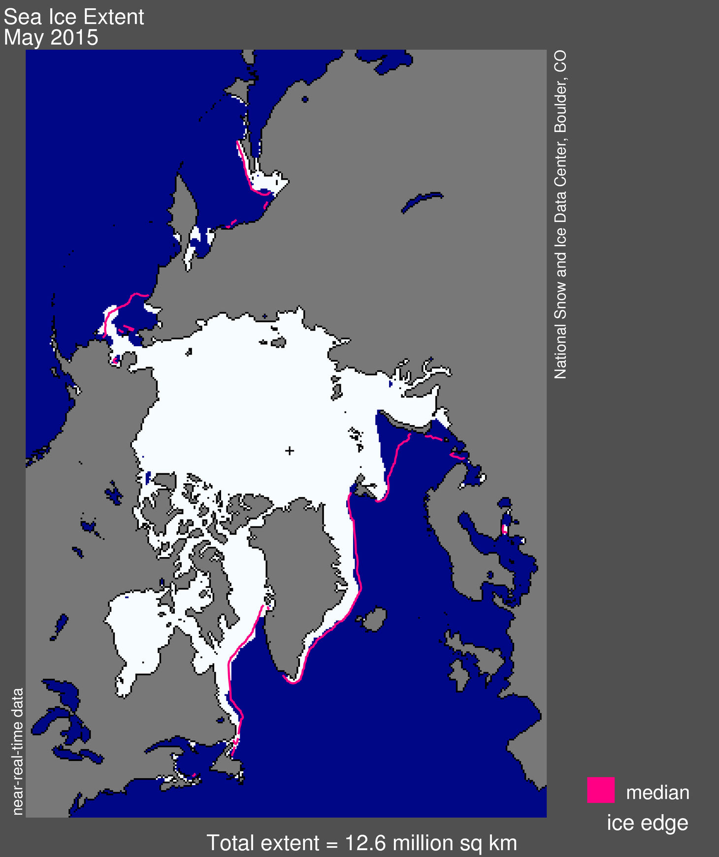
Figure 1. Arctic sea ice extent for May 2015 was 12.65 million square kilometers (4.88 million square miles). The magenta line shows the 1981 to 2010 median extent for that month. The black cross indicates the geographic North Pole. Sea Ice Index data. About the data
Credit: National Snow and Ice Data Center
High-resolution image
Arctic sea ice extent for May 2015 averaged 12.65 million square kilometers (4.88 million square miles), the third lowest May ice extent in the satellite record. This is 730,000 square kilometers (282,000 square miles) below the 1981 to 2010 long-term average of 13.38 million square kilometers (5.17 million square miles) and 70,000 square kilometers (27,000 square miles) above the record low for the month, observed in 2004.
The below average extent for this month is partly a result of early melt out of ice in the Bering Sea and the persistence of below-average ice conditions in the Barents Sea. Early breakup of sea ice in the Bering Sea also occurred last spring. Elsewhere, ice is tracking at near-average levels. By the end of May, several openings had appeared in the ice pack, most notably in the southern Beaufort Sea near Banks Island, off the coast of Barrow, Alaska, and in the Kara Sea. Now that we are entering the month of June, the rate of ice loss is likely to quicken, but how fast will depend on the weather conditions and the date of ice surface melt onset across the high Arctic.
Conditions in context
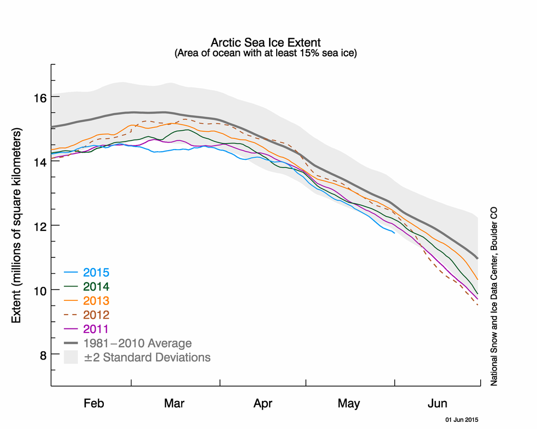
Figure 2a. The graph above shows Arctic sea ice extent as of June 1, 2015, along with daily ice extent data for four previous years. 2015 is shown in blue, 2014 in green, 2013 in orange, 2011 in brown, and 2011 in purple. The 1981 to 2010 average is in dark gray. The gray area around the average line shows the two standard deviation range of the data. Sea Ice Index data.
Credit: National Snow and Ice Data Center
High-resolution image
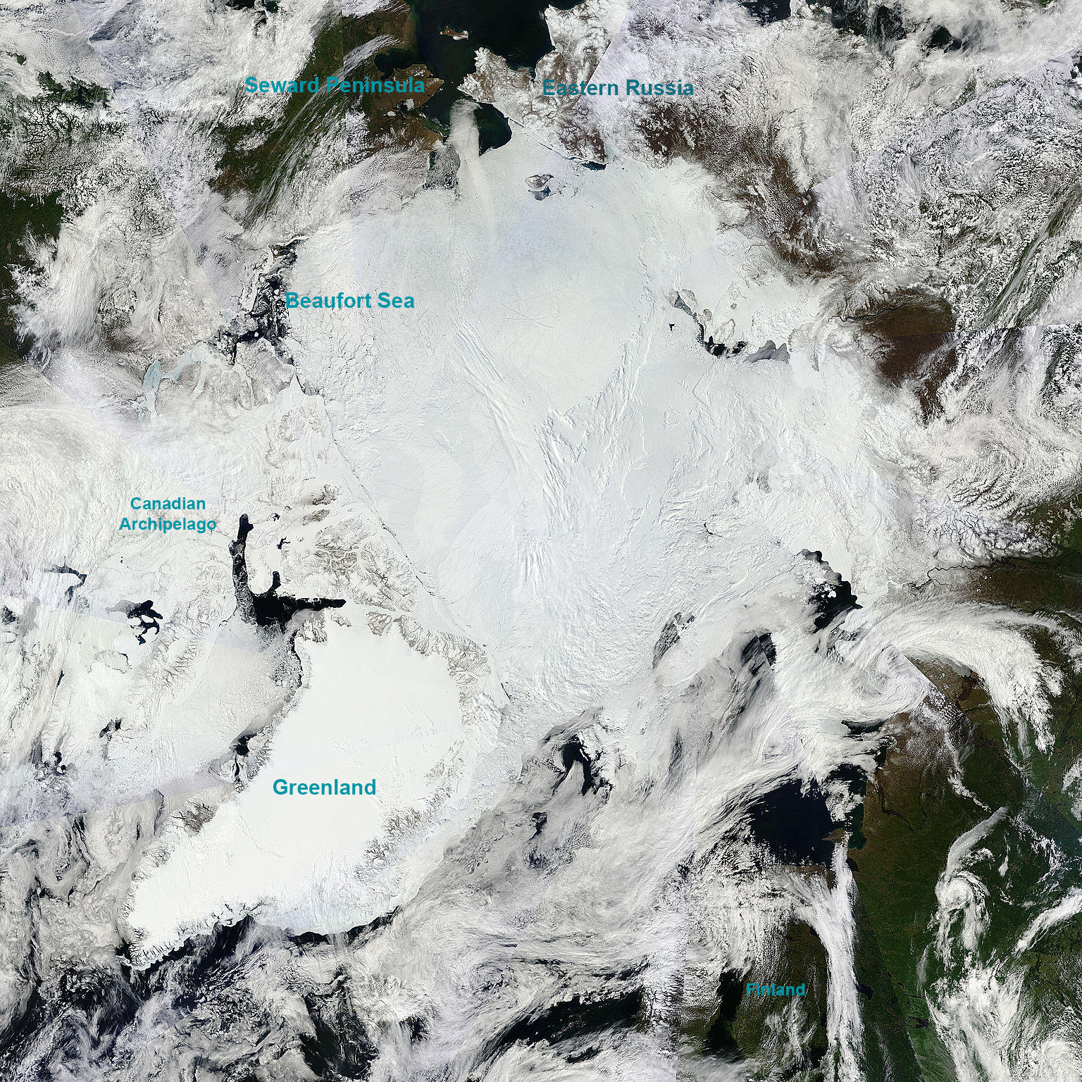
Figure 2b. In this satellite image, captured on June 2, 2015, broken up ice over the eastern Beaufort Sea is apparent. Eastern Russia is snow covered, while the Seward Peninsula is relatively snow free. Sea level pressures were high over the Arctic Ocean at this time. Greenland is seen clearly at the lower left. Image from the Moderate Resolution Imaging Spectroradiometer (MODIS) on the NASA Terra satellite.
Credit: Land Atmosphere Near-Real Time Capability for EOS (LANCE) System, NASA/GSFC
High-resolution image
Overall, May was cooler than average over the central Arctic Ocean, the East Greenland Sea and the East Siberian and Laptev seas, notably north of the Greenland Ice Sheet where air temperatures at the 925 millibar level (about 3,000 feet above the surface) were 2 to 4 degrees Celsius (4 to 7 degrees Fahrenheit) below average. However, temperatures were 4 to 8 degrees Celsius (7 to 14 degrees Fahrenheit) above average in the Beaufort Sea and the Barents and Kara seas, with surface temperatures rising above the freezing point in Barrow, Alaska. These temperature patterns were linked to below-average sea level pressures over the Bering Sea, Baffin Bay and the North Atlantic, coupled with above average pressures over Siberia, Alaska, and Canada. Associated wind patterns also helped to push ice offshore from the coast of Alaska, leading to the formation of open water off the coast of Barrow, Alaska.
Temperature conditions during May may prove to be important, given the potential role that melt ponds in spring play in the evolution of the ice cover throughout summer. For example, during years with fewer melt ponds in May, September sea ice extent tends to be higher than during years with more melt ponds. (See our May 2014 discussion of the importance of spring melt ponds.)
Overall the total ice extent for May 2015 declined at a fairly rapid pace, losing 1.69 million square kilometers (653,000 square miles). This was slightly faster than the 1981 to 2010 average rate of decline of 1.41 million square kilometers (544,000 square miles). The ice extent is now tracking at more than two standard deviations below the 1981 to 2010 long-term average.
May 2015 compared to previous years
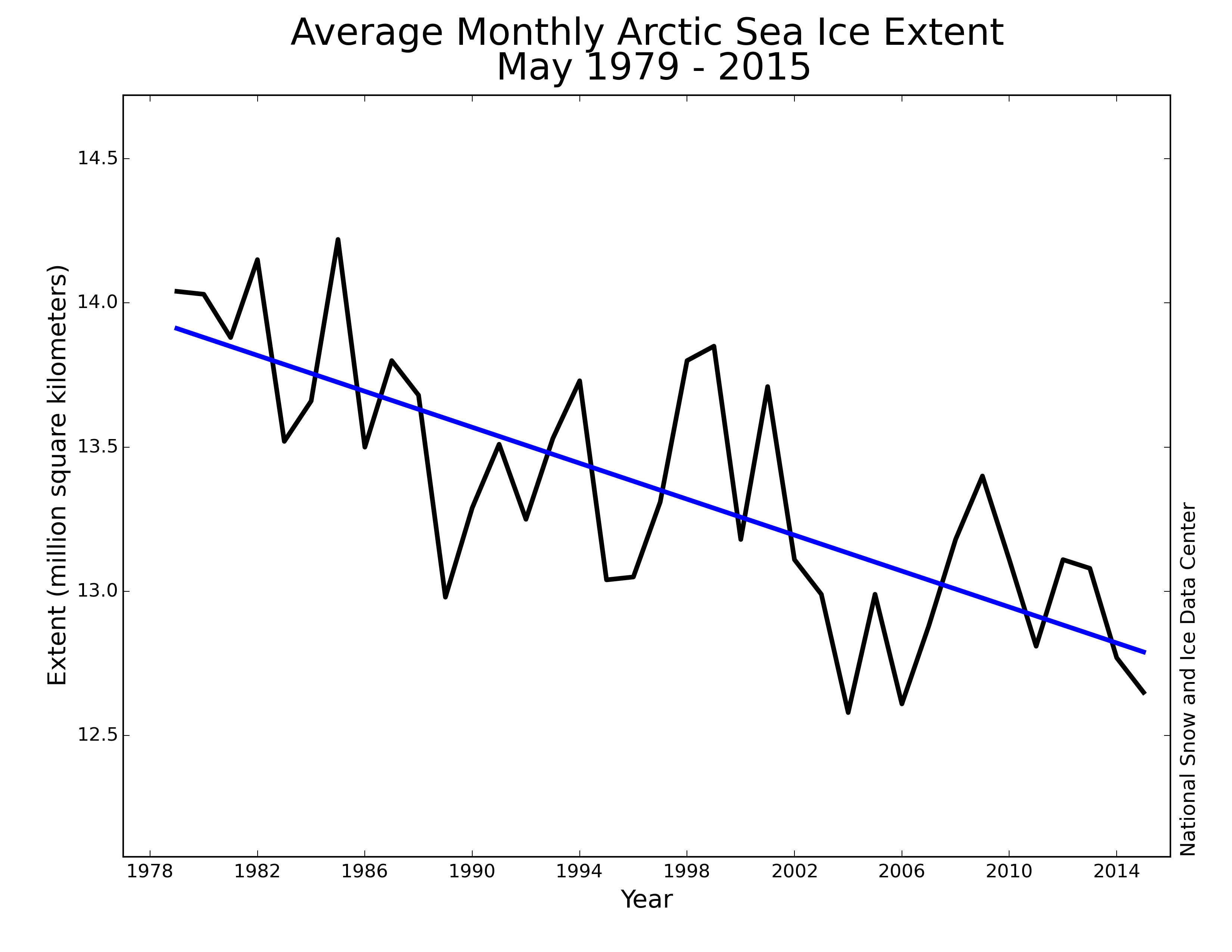
Figure 3. Monthly May ice extent for 1979 to 2015 shows a decline of 2.33% per decade relative to the 1981 to 2010 average.
Credit: National Snow and Ice Data Center
High-resolution image
Arctic sea ice extent averaged for May 2015 was the third lowest in the satellite record for the month. Through 2015, the linear rate of decline for May extent is 2.33% per decade.
Weather versus preconditioning
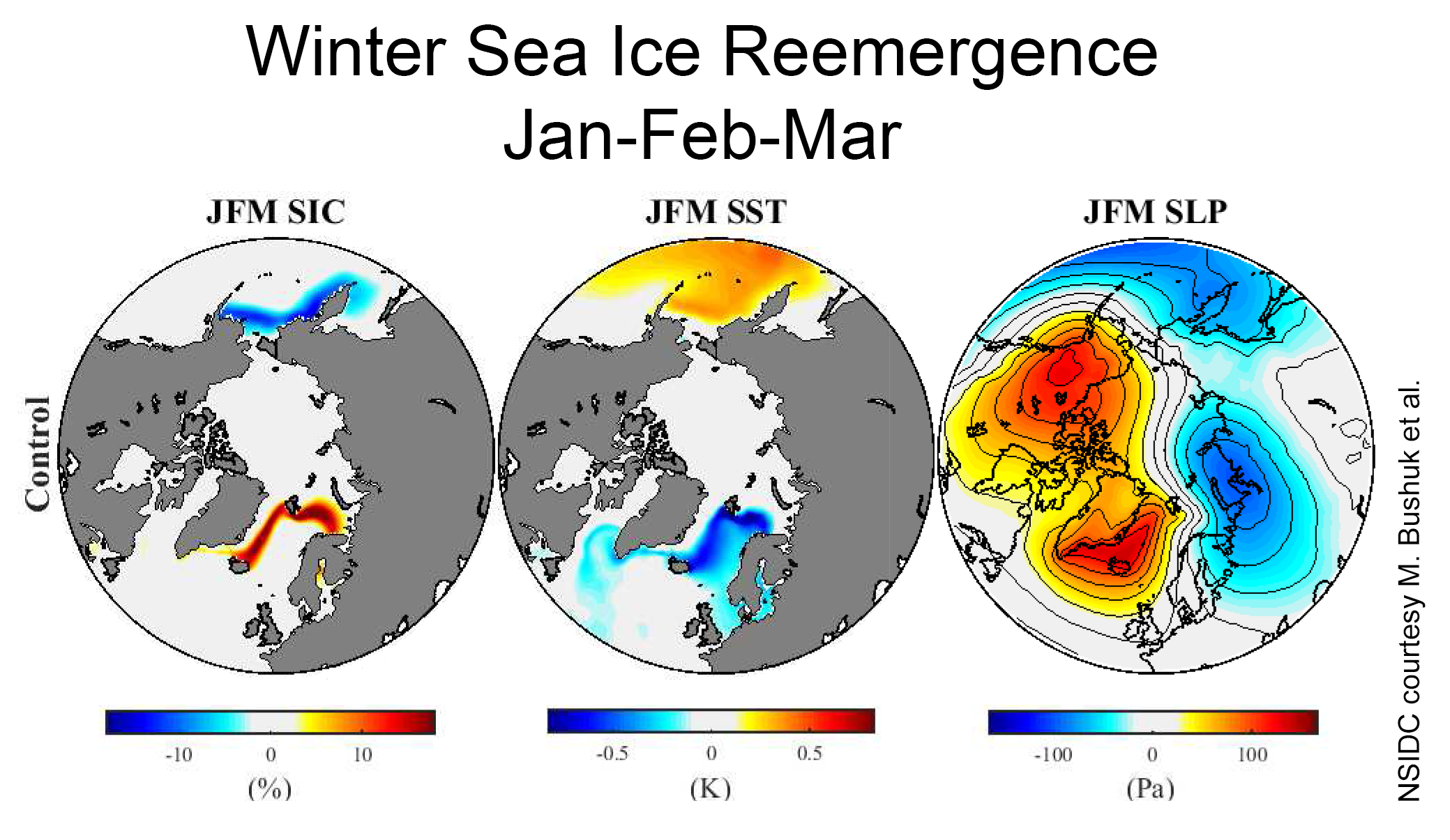
Figure 4. The images above compare patterns of winter (January-February-March) sea ice concentration anomalies (SIC, in percent concentration) with sea surface temperature anomalies (SST, in Kelvin) and sea level air pressures (SA, in pressure altitude), for a pre-industrial control model simulation.
Credit: M. Bushuk et al., Geophys. Res. Lett.
High-resolution image
The shrinking summer sea ice cover has fostered increased socioeconomic activity in the Arctic, such as resource extraction and ship traffic, leading to a focus on developing reliable methods to predict the summer minimum sea ice extent several months in advance.
Key to improving our ability to accurately forecast September sea ice conditions is a better understanding of the physical mechanisms underlying sea ice variability from year to year. An area of growing interest is sea ice reemergence: the observation that lower-than-average or higher-than-average sea ice extent tends to recur at time lags of 5 to 12 months. This reemergence phenomenon appears to be related to sea surface temperatures in the seasonal ice zones (from melt season to growth season), sea ice thickness in the central Arctic (from growth season to melt season) and atmospheric circulation (from melt season to growth season).
For example, a new study shows that when winter sea ice concentrations are above average in the East Greenland, Barents and Kara seas, ice concentrations tend to be below average in the Bering Sea. This spatial pattern of anomalies linking the North Atlantic and North Pacific is related to the sea level pressure pattern that drives surface winds and their associated movement of atmospheric heat. These conditions are in turn linked to cooler or warmer than average sea surface temperatures that provide memory, influencing regional sea ice concentrations the following autumn. Thus, while the atmosphere is critical in setting the spatial patterns of sea ice variability, the ocean provides the memory for reemergence.
Figure 4 shows the leading winter (January-February-March) patterns of sea ice reemergence in the Arctic, based on model output from a pre-industrial control simulation of the Community Climate System Model version 4 (CCSM4). The reemerging sea ice concentration (SIC) pattern is characterized by below-average SIC in the Bering Sea and above-average SIC in the Barents-Greenland-Iceland-Norwegian (Barents-GIN) seas. Local sea surface temperature anomalies (SSTs) have the opposite sign and provide memory that allows melt season SIC conditions to reemerge the following growth season. The sea level pressure (SLP) pattern drives winds that provide for communication between the North Atlantic and North Pacific.
The Sea Ice Prediction Network provides a forum for the sea ice forecasting community to share predictions of September mean sea ice extent using a variety of methods.
Down below, Antarctica above
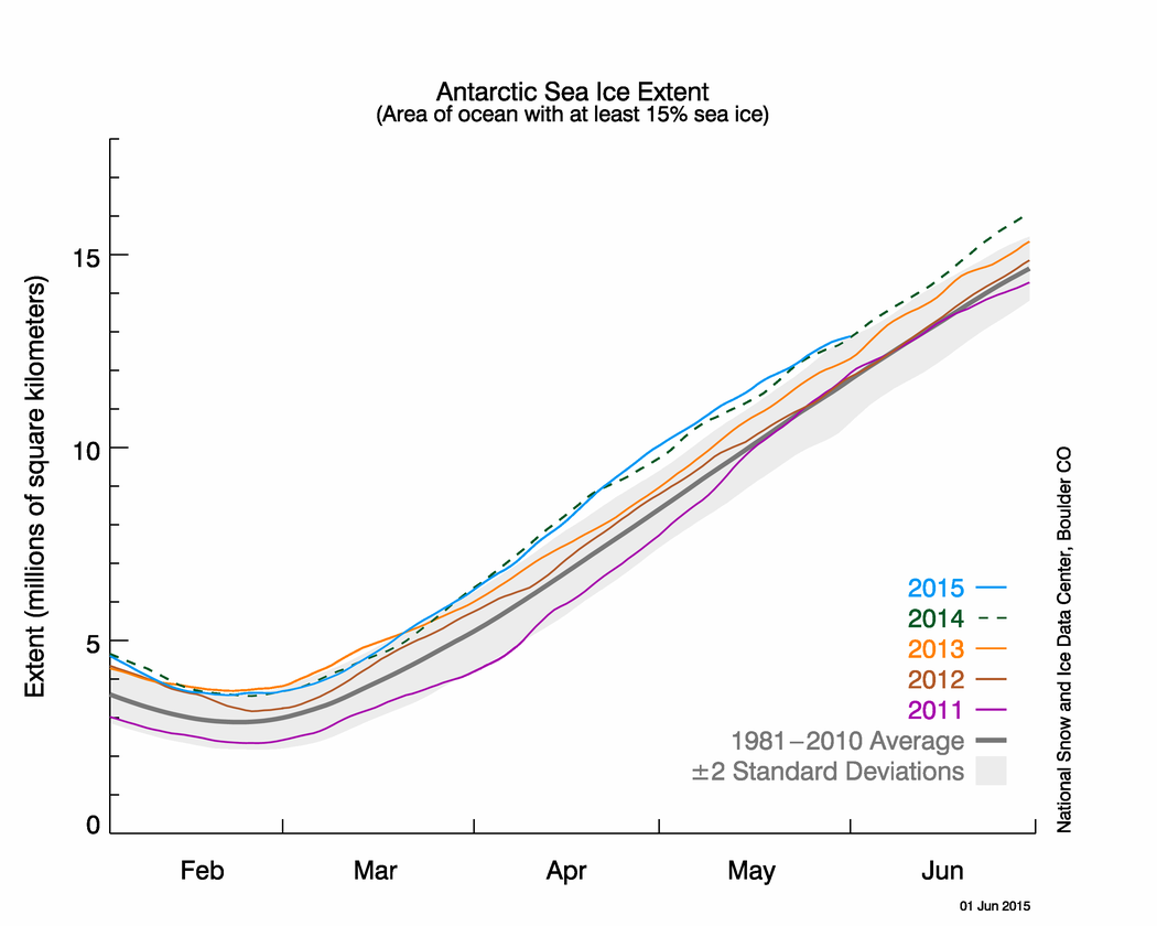
Figure 5. The graph above shows Antarctic sea ice extent as of June 1, 2015, along with daily ice extent data for four previous years. 2015 is shown in blue, 2014 in green, 2013 in orange, 2012 in brown, and 2011 in purple. The 1981 to 2010 average is in dark gray. The gray area around the average line shows the two standard deviation range of the data. Sea Ice Index data.
Credit: National Snow and Ice Data Center
High-resolution image
Beginning in late April, Antarctic sea ice extent surpassed the previous satellite-era record set in 2014, and for the entire month of May it has set daily record high ice extents. This makes May 2015 the record high month for the 1979 to 2015 period. As has been the case for several months, ice extent is unusually high in areas of the eastern Ross Sea – western Amundsen Sea, and in the northern and northeastern Weddell Sea. Unusually high extent has developed over the Davis Sea area of the far southern Indian Ocean.
Antarctic sea ice extent for May 2015 averaged 12.10 million square kilometers (4.67 million square miles). The linear rate of increase for May is now 2.88% per decade for the period 1979 to 2015.
Despite the record sea ice extent, air temperatures at the 925 millibar level (about 3,000 feet above the surface) remained generally above average for most of the continent and coastal areas of the surrounding ocean. Air temperatures were as much as 5 degrees Celsius (9 degrees Fahrenheit) above the 1981 to 2010 average over the West Antarctic ice sheet and central Ross Sea. The region of high ice extent near the northeastern Ross Sea had near-average air temperatures in the vicinity of the ice edge. Cooler than average temperatures were observed near the ice edge in the northeastern Weddell Sea (2 degrees Celsius, or 4 degrees Fahrenheit, below average) and Davis Sea (4 degrees Celsius, or 7 degrees Fahrenheit, below average). Air circulation patterns were variable for the month. The Southern Annular Mode, a north-south movement of the westerly wind belt that circles Antarctica, was in a near neutral state for the month as a whole.
Further reading
Bushuk, M., D. Giannakis, and A. J. Majda (2015). Arctic sea-ice reemergence: The role of large-scale oceanic and atmospheric variability. J. Climate, doi:10.1175/JCLI-D-14-00354.1, in press.
Bushuk, M. and D. Giannakis (2015). Sea-ice reemergence in a model hierarchy. Geophys. Res. Lett., doi:10.1002/2015GL063972, in press.
Schroeder, D., D.L. Feltham, D. Flocco and M. Tsmados, (2014). September Arctic sea ice minimum predicted by spring melt pond fraction. Nature Climate Change, doi:10.1038/nclimate2203.
Stroeve, J., E. Blanchard-Wrigglesworth, V. Guemas, S. Howell, F. Massonnet and S. Tietsche, (2015). Developing user-oriented seasonal sea ice forecasts in a changing Arctic. EOS, doi:10.1175/JCLI-D-14-00354.1, in press.

