While Arctic sea ice extent is increasing, total ice extent remains below average, tracking almost two standard deviations below the long-term average.
Overview of conditions
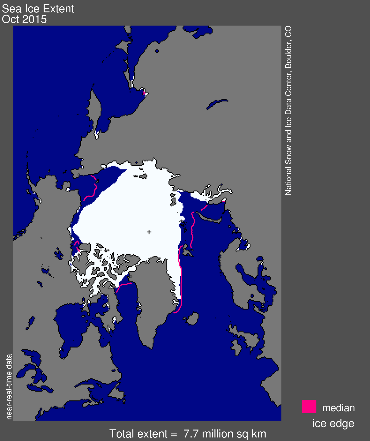
Figure 1. Arctic sea ice extent for October 2015 was 7.72 million square kilometers (2.98 million square miles). The magenta line shows the 1981 to 2010 median extent for that month. The black cross indicates the geographic North Pole. Sea Ice Index data. About the data
Credit: National Snow and Ice Data Center
High-resolution image
Arctic sea ice extent for October 2015 averaged 7.72 million square kilometers (2.98 million square miles), the sixth lowest October in the satellite record. This is 1.19 million square kilometers (460,000 square miles) below the 1981 to 2010 average extent, and 950,000 square kilometers (367,000 square miles) above the record low monthly average for October that occurred in 2007.
Conditions in context
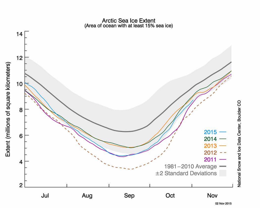
Figure 2. The graph above shows Arctic sea ice extent as of November 2, 2015, along with daily ice extent data for four previous years. 2015 is shown in blue, 2014 in green, 2013 in orange, 2012 in brown, and 2011 in purple. The 1981 to 2010 average is in dark gray. The gray area around the average line shows the two standard deviation range of the data. Sea Ice Index data.
Credit: National Snow and Ice Data Center
High-resolution image
Air temperatures at the 925 millibar level were 4 to 5 degrees Celsius (7 to 9 degrees Fahrenheit) above average over the central Arctic, extending towards Fram Strait. This appears to be due to unusually low pressure over northwest Greenland and higher pressures over the Tamyr Peninsula and Scandinavia, which funneled warm air from the south into the central Arctic Ocean. Coastal regions were generally 1 to 3 degrees Celsius (2 to 5 degrees Fahrenheit) higher than average.
October 2015 compared to previous years
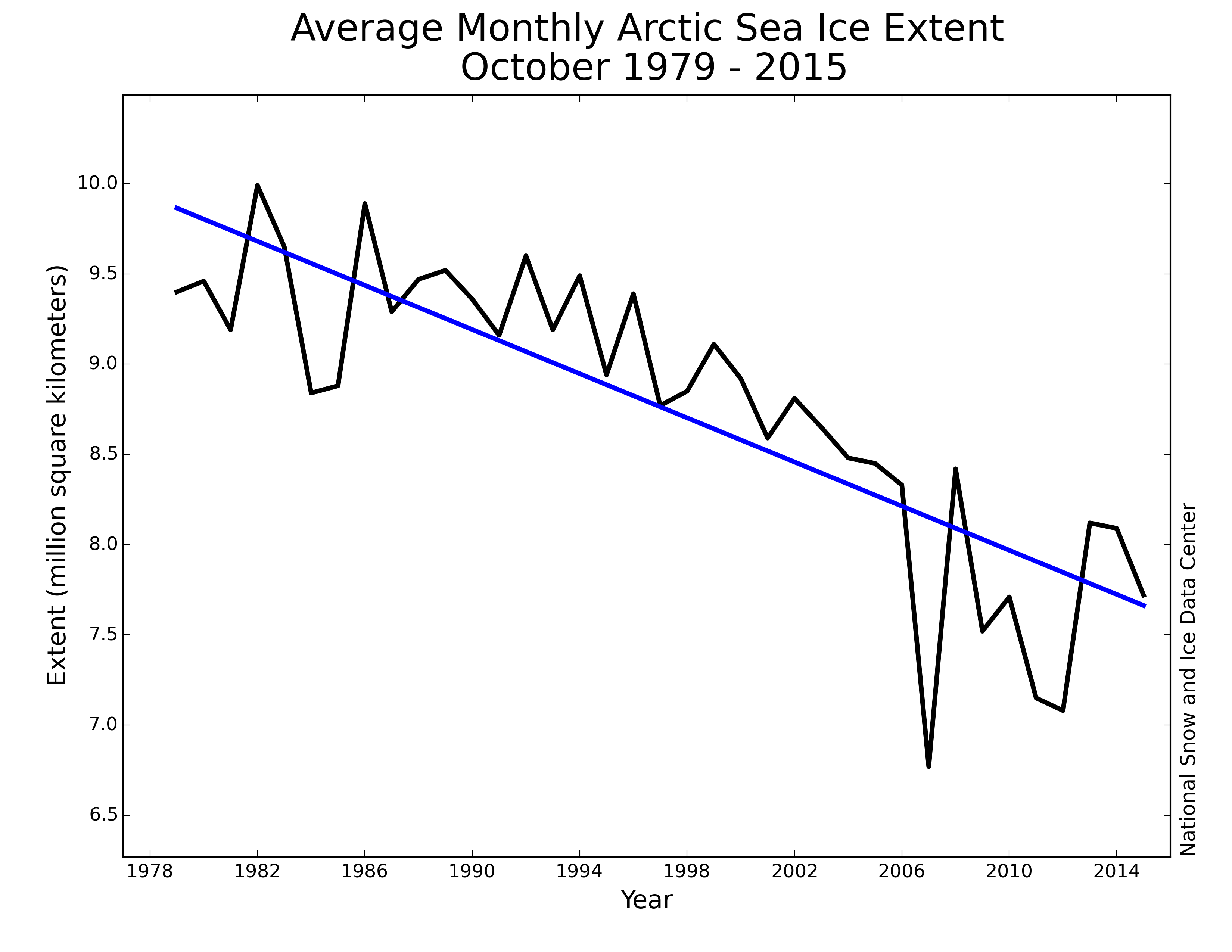
Figure 3. Monthly October ice extent for 1979 to 2015 shows a decline of 6.9% per decade.
Credit: National Snow and Ice Data Center
High-resolution image
Through 2015, the October sea ice extent has declined 6.9% per decade over the satellite record.
New sea ice thickness information back for the winter

Figure 4a. This image from CryoSat-2 shows thin ice (less than 1 meter, or 3 feet, thick) over a wide area north of Greenland.
Credit: Center for Polar Observation and Modeling (CPOM) at University College London
High-resolution image
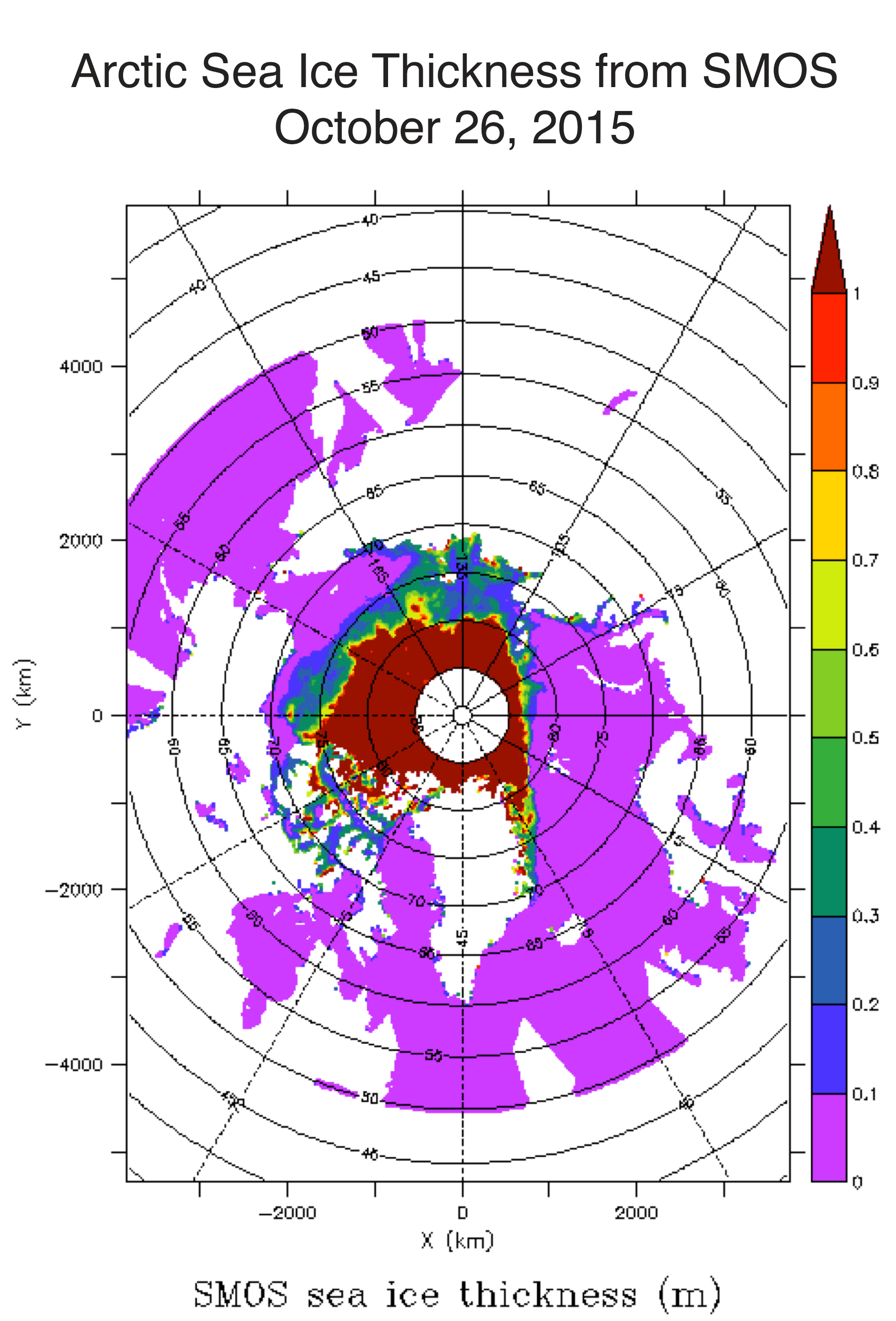
Figure 4b. This image from the European Space Agency’s Soil Moisture and Ocean Salinity (SMOS) satellite shows sea ice thickness over the Arctic Ocean.
Credit: University of Hamburg Integrated Climate Data Center
High-resolution image
In recent years, two European Space Agency (ESA) satellites, CryoSat-2 and SMOS (Soil Moisture and Ocean Salinity), have been providing information on sea ice thickness. Thickness information is valuable for assessing the overall condition of the sea ice cover. The sensors on these satellites cannot determine thickness during the summer melt season, but now that freeze-up has begun, information is again available.
CryoSat-2, launched in 2010, is a radar altimeter, which measures the height of the ice cover above the sea surface. Used with additional information on snow cover and its density, the height information can be converted into estimates of ice thickness. The Center for Polar Observation and Modeling (CPOM) at University College London has again started providing near-real-time maps of sea ice thickness from CryoSat-2.
While these maps are valuable in providing near-real-time thickness estimates, converting the satellite measurements into thickness involves complex processing and there are many uncertainties. For example, Figure 4a depicts thin ice (less than 1 meter [3 feet]) over a wide area north of Greenland, an area where wind and ocean current patterns push the ice against the coast forming thick ridges and an extremely rough surface. This area has been shown by other studies to have some of the thickest sea ice in the Arctic, often exceeding 4 meters (13 feet). This ridging may have cause the difficulty in the current mapping.
CryoSat-2 also has difficulty retrieving thickness in very thin sea ice regions, resulting in no thickness values reported at the outer edge of the ice cover. SMOS is a microwave imaging radiometer that measures microwave brightness temperature at a range that is sensitive to thin ice (1.4 gigahertz). These data are also now available in near-real-time at the University of Hamburg Integrated Climate Data Center. SMOS cannot estimate thickness beyond 1 meter (3.28 feet) at most and often not beyond 0.5 meters (1.64 feet). While the map shows a wide region of 1 meter-thick ice, it is important to realize that this is just the maximum allowable value and in reality there is thicker ice over much of the region. However, SMOS provides valuable information on the coverage of thin ice during the winter ice growth season. Ideally, a blended CryoSat-2/SMOS product will provide more comprehensive information on thickness.
A large ozone hole over the Antarctic

Figure 5. The image above shows the ozone hole over Antarctica on October 2, 2015 when it had reached its largest single-day area for the year, spanning 28.2 million square kilometers (10.9 million square miles). Data are from the Ozone Monitoring Instrument (OMI) on the NASA Aura satellite and the Ozone Monitoring and Profiler Suite (OMPS) on the NASA-NOAA Suomi NPP satellite.
Credit: NASA Earth Observatory, Ozone Hole Watch
High-resolution image
While sea ice in Antarctica is near average, the ozone hole over the continent grew relatively large during the austral winter. This goes against the expected trend towards a smaller ozone hole since the use of chlorofluorocarbons (CFCs) was banned in 1996. The size of the hole in a given year depends on several factors, including temperatures in the high altitude stratosphere. Temperatures in the Antarctic stratosphere were low this year, aiding chemical processes that destroy ozone. For more information on this year’s ozone hole see this NASA Earth Observatory feature.

