After reaching near-average levels in late April, sea ice extent declined rapidly during the early part of May. The rest of the month saw a slower rate of decline. Ice extent in the Bering Sea remained above average throughout the month.
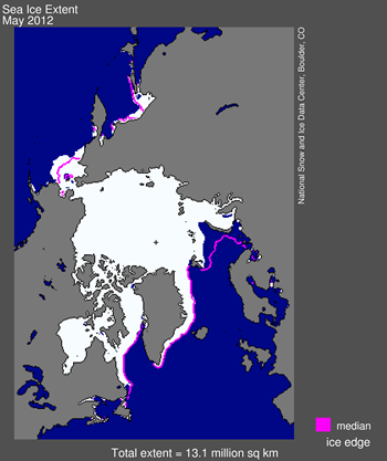
Figure 1. Arctic sea ice extent for May 2012 was 13.13 million square kilometers (5.07 million square miles). The magenta line shows the 1979 to 2000 median extent for that month. The black cross indicates the geographic North Pole. Sea Ice Index data. About the data
Credit: National Snow and Ice Data Center
High-resolution image
Overview of conditions
Arctic sea ice extent for May 2012 averaged 13.13 million square kilometers (5.07 million square miles). This was 480,000 square kilometers (185,000 square miles) below the 1979 to 2000 average extent. This May’s extent was similar to the May 2008 – 2010 extent, but it was higher than May 2011. May ice extent was 550,000 square kilometers (212,000 square miles) above the record low for the month, which happened in the year 2004.
Ice cover remained extensive in the Bering Sea, continuing the pattern observed this past winter and spring. The anomalously heavy ice conditions were countered by unusually low extents in the Barents and Kara Seas, resulting in Arctic-wide ice conditions that remained below normal. By the end of the month, open water areas had begun to form along some parts of Arctic Ocean coast.
While the ice extent for May is not especially low this year, there is little correlation between the extent of the ice cover in May and that at the end of the melt season in September.

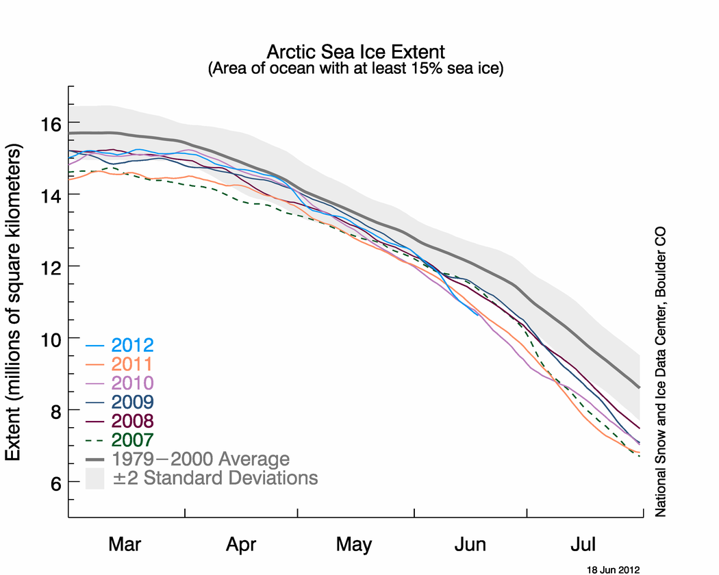
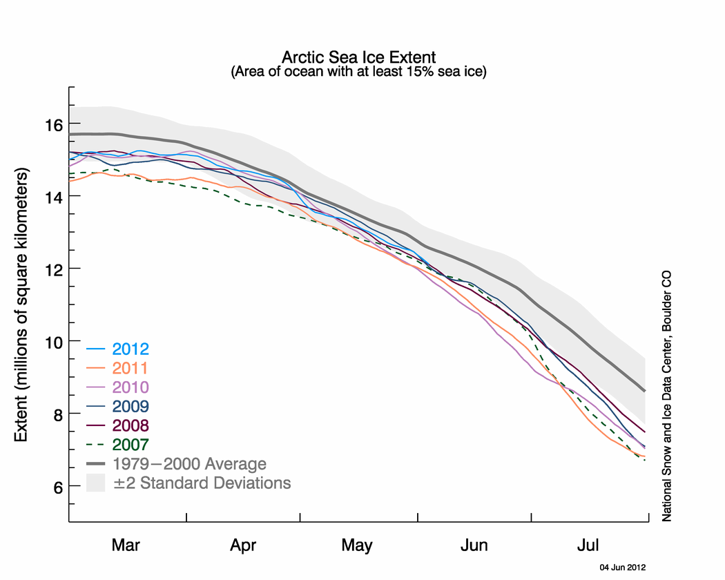
Figure 2. The graph above shows Arctic sea ice extent as of June 4, 2012, along with daily ice extent data for the previous five years. 2012 is shown in blue, 2011 in orange, 2010 in pink, 2009 in navy, 2008 in purple, and 2007 in green. The gray area around the average line shows the two standard deviation range of the data. Sea Ice Index data.
Credit: National Snow and Ice Data Center
High-resolution image
Conditions in context
For May, the Arctic as a whole lost 1.62 million square kilometers (625,000 square miles) of ice, which was 180,000 square kilometers (69,500 square miles) more than the 1979 to 2000 average. The average daily rate of ice loss was 52,000 square kilometers (20,000 square miles) per day, which was slightly faster than the long-term average of 46,000 square kilometers (18,000 square miles) per day. However, the rate of ice loss for the month was composed of two distinct periods: a rapid loss of ice during the first part of the month, followed by near-average rates during the latter part of the month.
Air temperatures for May were higher than usual over the central Arctic Ocean and the Canadian Archipelago. Over the Bering Sea, Hudson Bay, and parts of the East Greenland and Norwegian seas, temperatures were slightly below average.
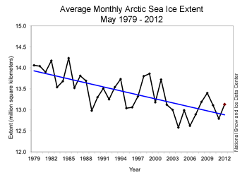
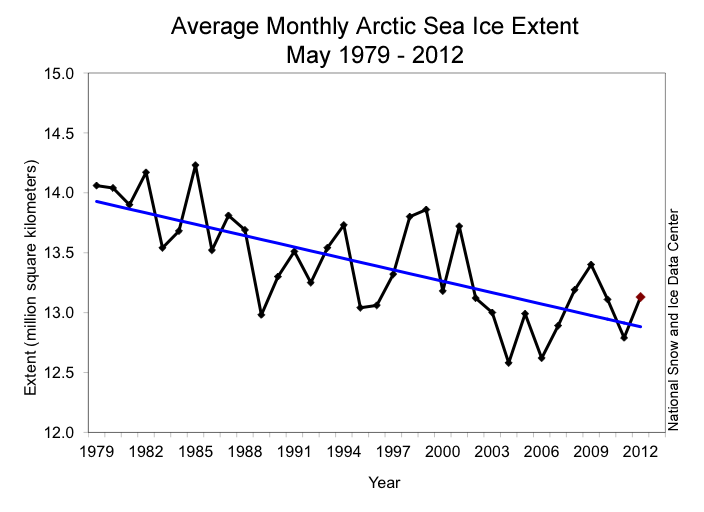
Figure 3. Monthly May ice extent for 1979 to 2012 shows a decline of 2.3% per decade.
Credit: National Snow and Ice Data Center
High-resolution image
May 2012 compared to past years
Arctic sea ice extent for May 2012 was below average for the month, compared to the satellite record from 1979 to 2000. However, the ice extent this May was not as low as it has been in some recent years. Including the year 2012, the linear rate of decline for May ice extent over the satellite record is 2.3% per decade.
May and April have the smallest trends of the year, indicating that spring is a period during the year when there is less variability and conditions tend to converge. It also demonstrates that spring extents are not necessarily indicative of conditions later in the summer.
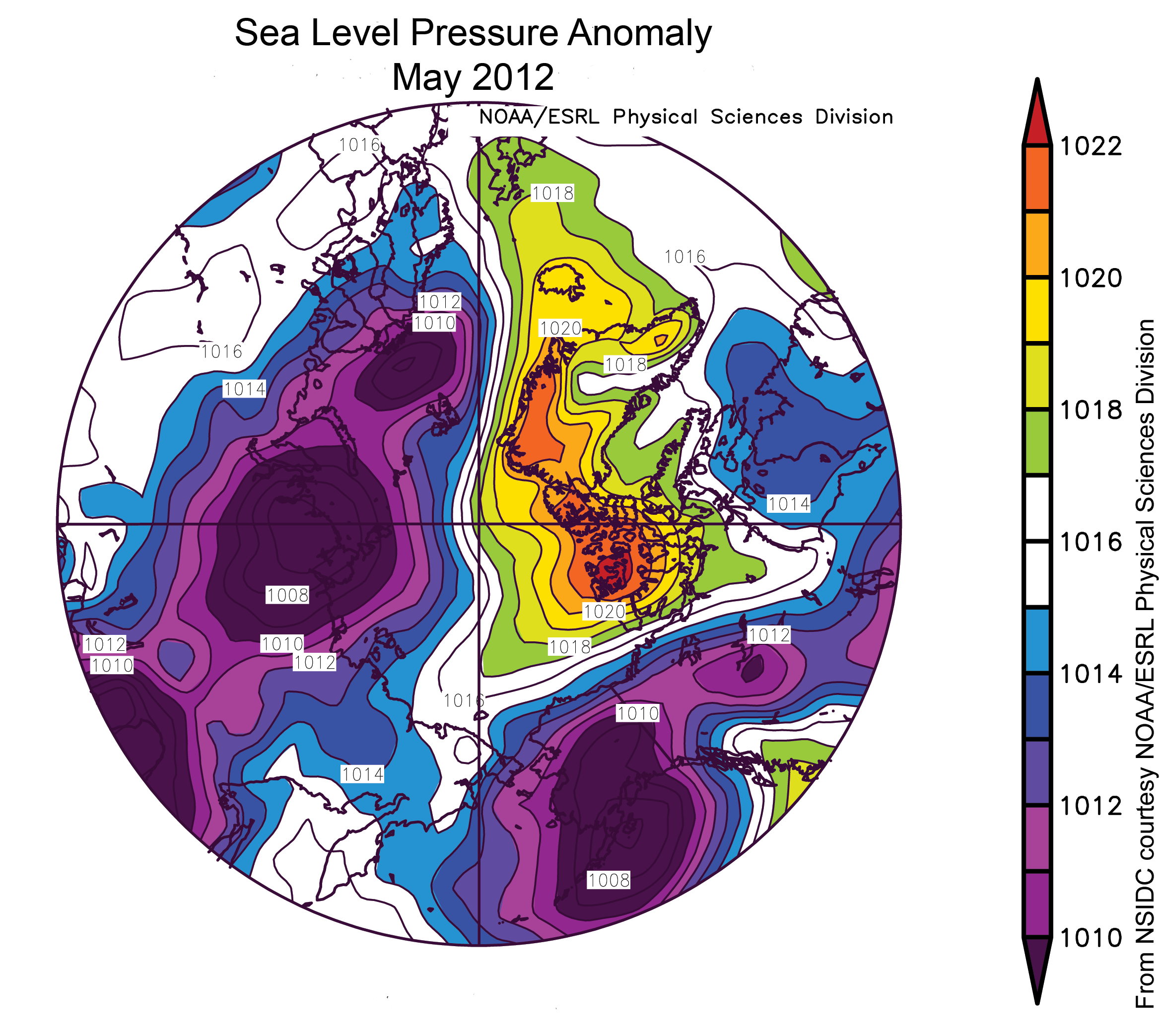
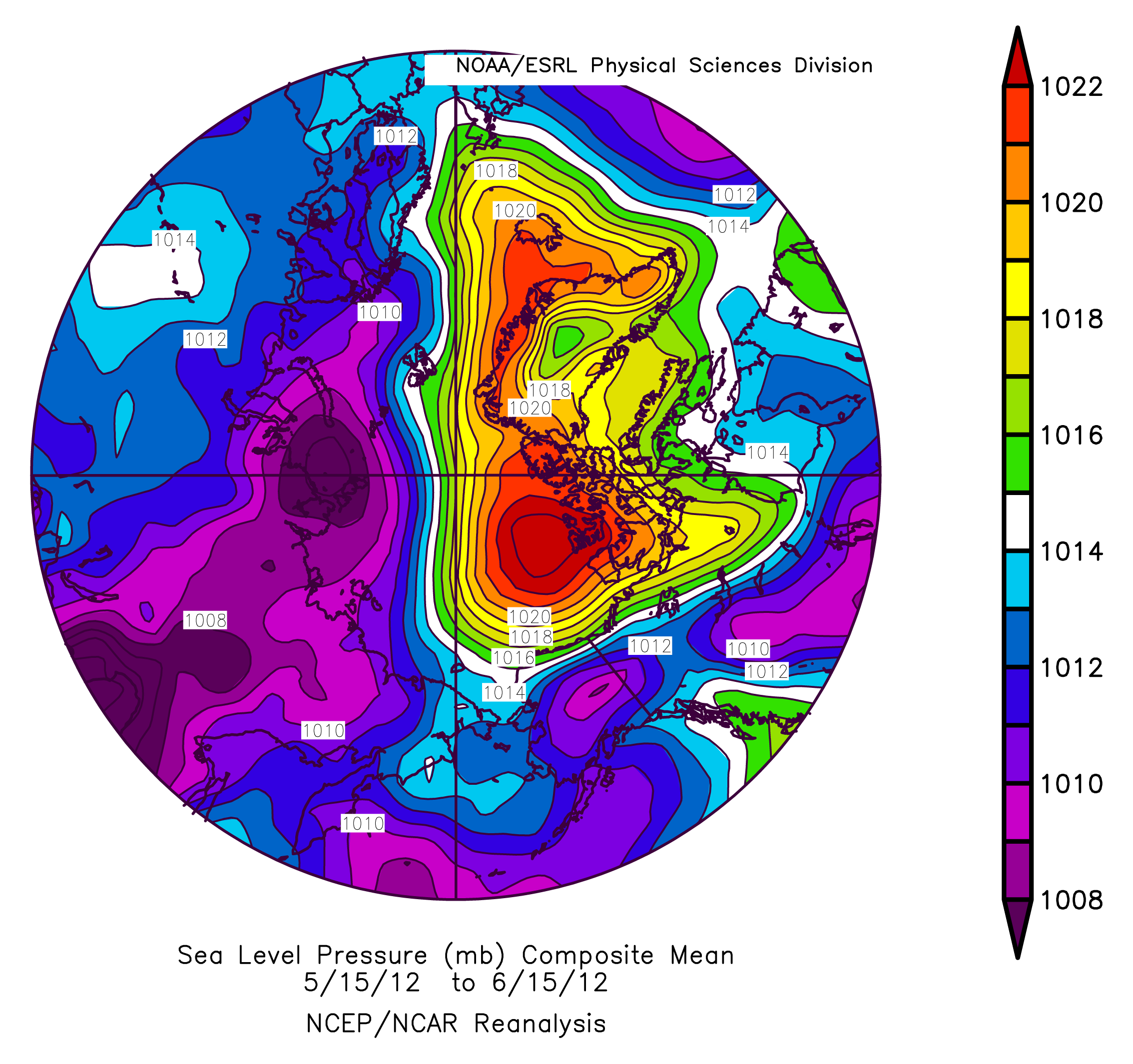
Figure 4. This map of sea level pressure anomalies for May 2012 shows that low pressure continued to dominate off of southern Alaska, resulting in northerly winds in the Bering Sea.
Credit: NSIDC courtesy NOAA/ESRL PSD
High-resolution image
A persistent pattern of extensive ice in the Bering Sea
Continuing the pattern of the past six months, ice cover remained unusually extensive in the Bering Sea. Normally by the end of May, the Bering is largely ice-free, but this year, 350,000 square kilometers (135,000 square miles) of ice remained. As was also the case for February through April, May 2012 had the highest average Bering Sea ice extent for the month in the satellite record.
The higher than normal extent and late spring break up of the ice cover in the Bering Sea are mainly due to unusually low air temperatures and persistent winds from the north, related to a region of low atmospheric pressure centered over Kodiak, Alaska. As these cold winds slowed ice melt, they also pushed the ice edge to the south. The heavy ice in the region may delay the start of Shell Alaska’s Arctic drilling this summer, which will be the first exploratory drilling in the Arctic Ocean in 20 years.
With the overall springtime warming of the Arctic, the ice has nevertheless started to break up and large areas of open water are now present in the northern part of the Bering Sea.

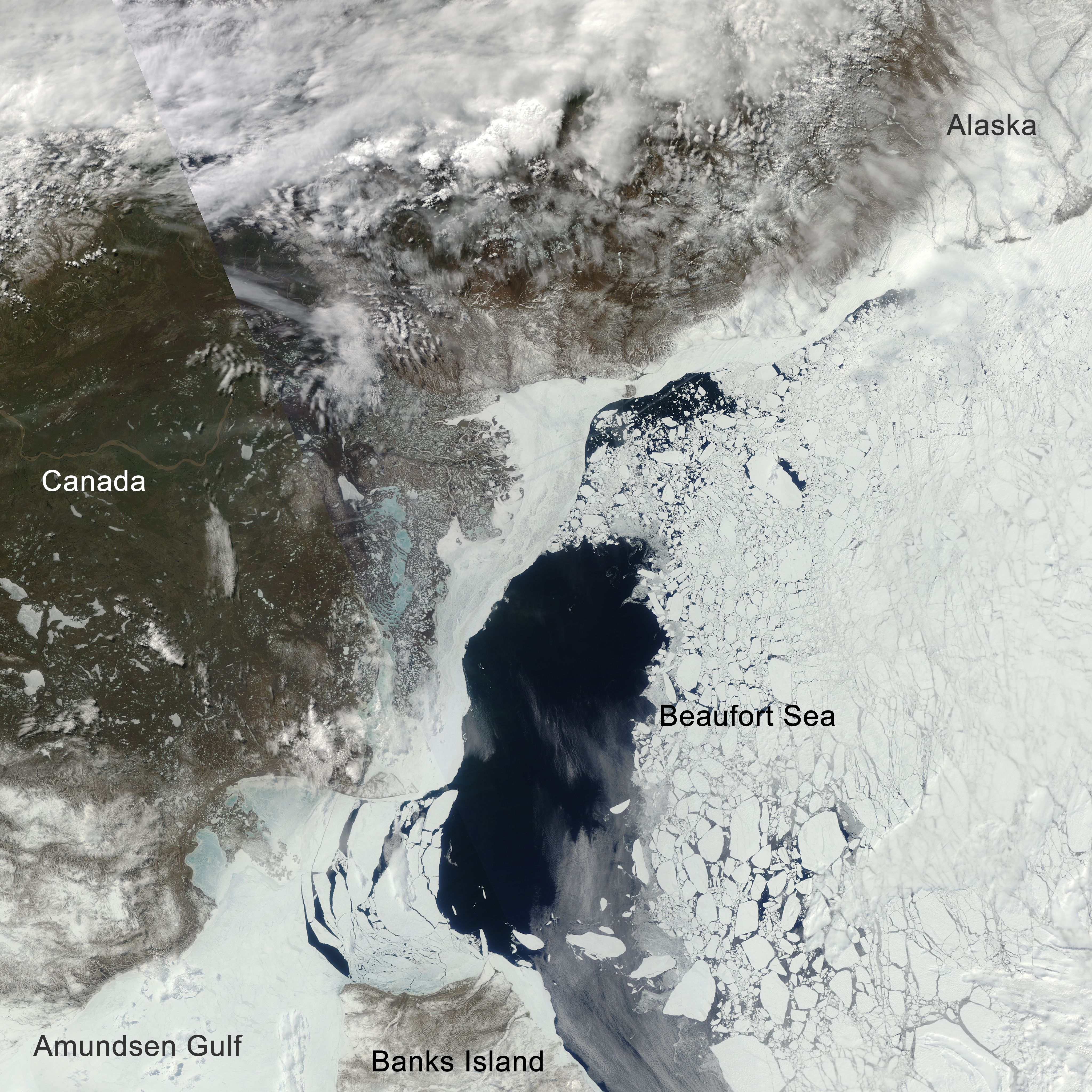
Figure 5. In this Moderate Resolution Imaging Spectroradiometer (MODIS) Arctic Mosaic image for the Beaufort Sea on May 29, 2012, open water is apparent between fast ice along the coast and the broken-up floes off-shore. Toward the bottom of the image, thin clouds can be seen over the open water.
Credit: NASA/GSFC, Rapid Response
High-resolution image
Open water areas within the Arctic Ocean
Although ice extent has remained high in the Bering Sea, open water areas have developed in parts of the Arctic Ocean, notably along the coasts of the Beaufort and Laptev seas. These openings are largely driven by winds pushing the ice away from fast ice, ice that is attached to the coast and that does not move with the winds. That the open water areas have not refrozen points to the relatively warm conditions over the Arctic, particularly in the Beaufort Sea.
The ice cover in the southern Beaufort Sea is also substantially broken up, with many individual ice floes instead of a consolidated pack. This makes the ice in this region vulnerable to enhanced melt during summer, as the sun rises higher in the sky and the dark open water areas between the floes readily absorb solar energy.
Quicker thickness data from NASA IceBridge
As we discussed last month, thickness information is extremely important for understanding the state of the ice cover. It is particularly important to seasonal forecasts (such as the SEARCH Sea Ice Outlook that will be released later this month), because thinner ice is more likely to melt completely during summer.
Sea ice age can be inferred from satellite data, and can help indicate the locations of relatively thin versus relatively thick ice. But direct measurements of ice thickness have been limited. Satellite missions such as ICESat and CryoSat, which measure ice thickness with altimeters, have been extremely valuable in better understanding overall changes in Arctic sea ice volume.
Currently, the NASA IceBridge mission supplies both sea ice thickness and snow depth measurements in spring, providing timely information on the state of the ice cover as the melt season begins. IceBridge data are collected from aircraft that fly over the ice cover carrying a suite of instruments, including altimeters that can directly measure ice thickness above the surface. These measurements are at high spatial resolution that can also be used to validate satellite data.
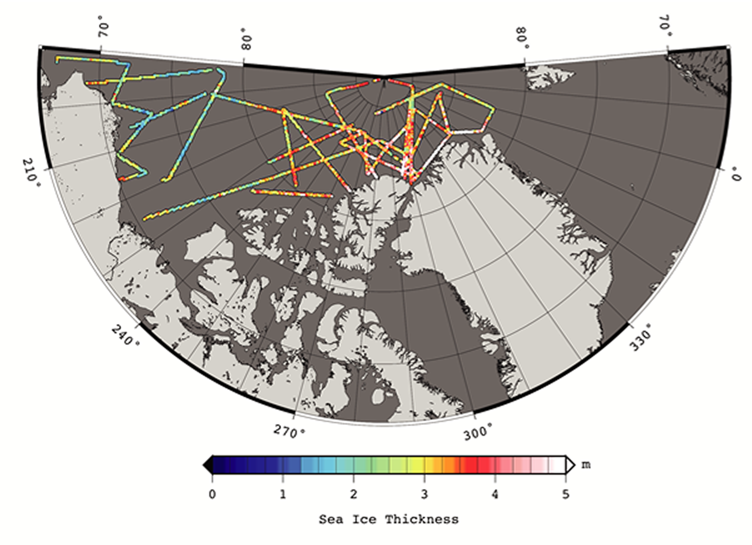
This year, the IceBridge Arctic sea ice campaign collected data in late March and early April, and provided data to NSIDC for distribution shortly thereafter. The data, collected from the North American side of the Arctic, indicate thick ice north of Greenland due to wind and ocean current patterns piling ice into thick ridges. In the Beaufort Sea, the offshore ice is fairly thin (1 to 2 meters, or 3 to 6 feet), indicative of first-year ice. Such thin ice will be prone to melt out completely this summer.
Ice along the Alaskan coast is thicker. Thicker ice tends to have a deeper overlying snow cover. The amount of snow is an important factor in the summer melt, because the snow reflects solar energy. The snow must melt away before surface melting of the ice can begin in earnest.


