Sea ice continues to track at low levels

Arctic sea ice continued to track at levels far below average through the middle of July, with open water in the Kara and Barents seas reaching as far north as typically seen during September. Melt onset began earlier than normal throughout most of the Arctic.

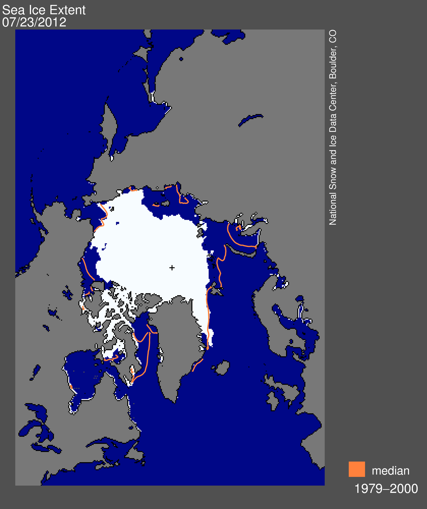
Figure 1. Arctic sea ice extent for July 23, 2012 was 7.32 million square kilometers (2.82 million square miles). The orange line shows the 1979 to 2000 median extent for that day. The black cross indicates the geographic North Pole. Sea Ice Index data. About the data

Credit: National Snow and Ice Data Center
High-resolution image

Overview of conditions
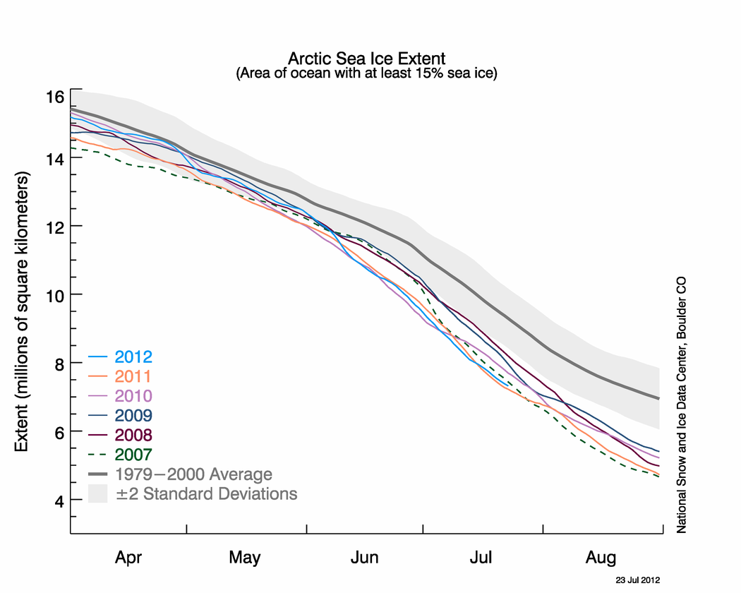
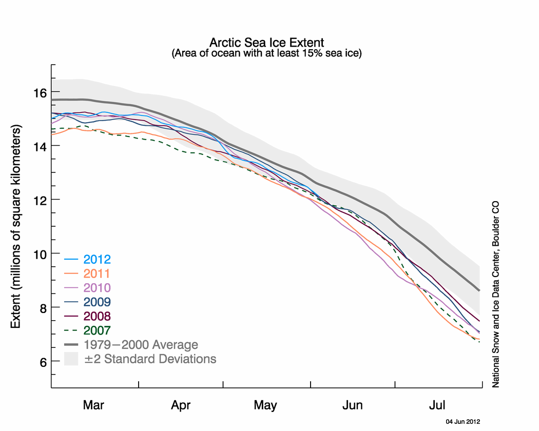
As of July 23, 2012, sea ice extent was 7.32 million square kilometers (2.82 million square miles). On the same day last year, ice extent was 7.22 million square kilometers (2.78 million square miles), the record low for this day.

Arctic sea ice extent continued to track at very low levels, setting daily record lows for the satellite era for a few days in early July. Extent is especially low in the Barents, Kara, and Laptev seas. In the Barents and Kara seas, the area of open water extends to the north coasts of Franz Josef Land and Severnaya Zemlya, as far north as typically seen during September, the end of the summer melt season. Polynyas in the Beaufort and East Siberian seas continued to expand during the first half of July. By sharp contrast, ice extent in the Chukchi Sea remains near normal levels. In this region the ice has retreated back to the edge of the multiyear ice cover. Ice cover in the East Greenland Sea, while of generally low concentration, remains slightly more extensive than normal.

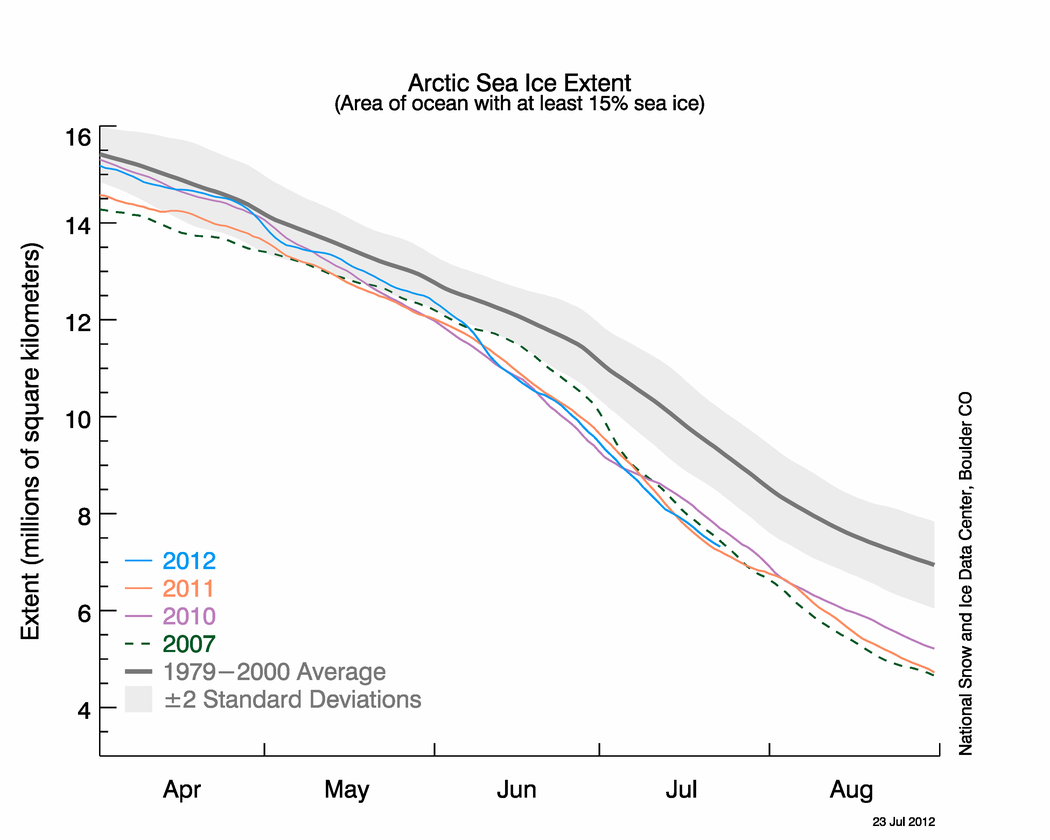
Figure 2. The graph above shows Arctic sea ice extent as of July 23, 2012, along with daily ice extent data for the previous five years. 2012 is shown in blue, 2011 in orange, 2010 in pink, 2009 in navy, 2008 in purple, and 2007 in green. The gray area around the average line shows the two standard deviation range of the data. Sea Ice Index data.

Credit: National Snow and Ice Data Center
High-resolution image

Conditions in context
The first part of July was once again dominated by high sea level pressure over the Beaufort Sea, combined with low sea level pressure over Siberia and Alaska. As discussed in last month’s post, this pressure pattern tends to promote above-average temperatures and enhances ice transport out of the Arctic through Fram Strait. Beginning July 11th, the pressure pattern changed as cyclones moved into the central Arctic Ocean, bringing in cooler temperatures and helping to slow ice loss. Air temperatures at the 925 hPa level (about 3000 feet) in the central Arctic and the Beaufort Sea were 1 to 4 degrees Celsius (2 to 7 degrees Fahrenheit) above normal as averaged from July 1 to July 14. In the Beaufort and Chukchi seas, the sea ice has retreated to the edge of the multiyear ice cover. As a result of the anomalously high air temperatures, melt over the multiyear ice cover is extensive and ice concentrations are low. Anomalously low air temperatures for that period were found in the Barents, Kara, and East Greenland seas (1 to 3 degrees Celsius, or 2 to 6 degrees Fahrenheit, below the 1981 to 2010 climatology).

Early melt onset
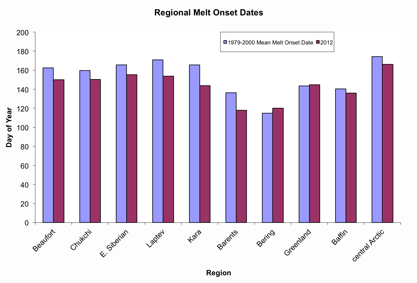
The timing of seasonal melt onset, which can be estimated from satellite passive microwave data, plays an important role in the amount of ice that melts each summer. Unusually early melt onset means an early reduction in the surface albedo, allowing for more solar heating of the ice, which in turn allows melt ponds and open water areas to develop earlier in the melt season. In 2012, melt began earlier than normal (as compared to averages for the period 1979 to 2000) throughout most of the Arctic, the exceptions being the Bering Sea and the East Greenland Sea. Melt in the Kara and Barents seas began more than two weeks earlier than normal. Melt onset for the Laptev Sea region as a whole started on June 1 and was the earliest seen in the satellite record. Melt began 12 and 9 days earlier than normal averaged over the Beaufort and Chukchi seas, respectively.

Figure 4. This composite image from the SSMIS instrument obtained on July 23, 2012 shows areas of low ice concentration in the Beaufort and Chukchi seas, the Canadian Archipelago, the East Greenland Sea, and north of Siberia. Purple indicates areas of high sea ice concentration, while yellow and red indicate lower ice concentration. Blue shows open water and green shows land.

Credit: National Snow and Ice Data Center courtesy IUP Bremen
High-resolution image

Low ice concentrations
NSIDC uses satellite data from the Special Sensor Microwave Imager (SSM/I) and the Special Sensor Microwave Imager/Sounder (SSMIS) instruments, in part because they provide the longest consistent time series of data. However, more recent sensors such as the Advanced Microwave Scanning Radiometer-Earth Observing System (AMSR-E) provide a more detailed perspective. In particular, we can examine ice concentration, which tells us how much ice is in a pixel, providing information on how vulnerable the ice may be to summer melting.

In October 2011, the AMSR-E instrument on board the NASA Aqua satellite ceased operation, dealing a blow to the science community. This is because its higher spatial resolution and advanced technology provided detailed ice information to complement the long-term record of the Special Sensor Microwave Imager/Sounder (SSMIS) instrument. However, the Japanese Aerospace Exploration Agency (JAXA) successfully launched a new satellite called Shizuku, or Global Change Observation Mission 1st-Water (GCOM-W1), on May 18, 2012. The Shizuku carries a new Advanced Microwave Scanning Radiometer (AMSR2) instrument, a sensor similar to AMSR-E. As soon as calibration and validation of AMSR2 are complete, the University of Bremen will once again produce maps of sea ice concentration at a fairly high resolution (about 6 kilometers).

In the meantime, the University of Bremen offers sea ice concentration maps from the lower-resolution SSMIS. The July 23 chart shows areas of low sea ice concentration in the Beaufort and Chukchi seas, the Canadian Archipelago, the East Greenland Sea, and north of Siberia. In the Beaufort and Chukchi seas, low ice concentrations and polynyas are found over areas of multiyear sea ice, where open water areas have developed between individual multiyear ice floes and significant ponding on the ice is observed. Low ice concentrations mean a low surface albedo, allowing for more of the sun’s energy to be absorbed, melting even more sea ice. This makes the multiyear ice in the Beaufort and Chukchi seas vulnerable to melting out this summer.

Rapid sea ice retreat in June

Arctic sea ice extent declined quickly in June, setting record daily lows for a brief period in the middle of the month. Strong ice loss in the Kara, Bering, and Beaufort seas, and Hudson and Baffin bays, led the overall retreat. Northern Hemisphere snow extent was unusually low in May and June, continuing a pattern of rapid spring snow melt seen in the past six years.

sea ice extent

Figure 1. Arctic sea ice extent for June 2012 was 10.97 million square kilometers (4.24 million square miles). The magenta line shows the 1979 to 2000 median extent for that month. The black cross indicates the geographic North Pole. Sea Ice Index data. About the data

Credit: National Snow and Ice Data Center
High-resolution image
Daily data files

Overview of conditions
Arctic sea ice extent for June 2012 averaged 10.97 million square kilometers (4.24 million square miles). This was 1.18 million square kilometers (456,000 square miles) below the 1979 to 2000 average extent. The last three Junes (2010-2012) are the three lowest in the satellite record. June 2012 ice extent was 140,000 square kilometers (54,000 square miles) above the 2010 record low. Ice losses were notable in the Kara Sea, and in the Beaufort Sea, where a large polynya has formed. Retreat of ice in the Hudson and Baffin bays also contributed to the low June 2012 extent. The only area of the Arctic where sea ice extent is currently above average is along the eastern Greenland coast.

The ice extent recorded for 30 June 2012 of 9.59 million square kilometers (3.70 million square miles) would not normally be expected until July 21, based on 1979-2000 averages. This puts extent decline three weeks ahead of schedule.

graph of sea ice extents

Figure 2. The graph above shows Arctic sea ice extent as of July 2, 2012, along with daily ice extent data for the previous five years. 2012 is shown in blue, 2011 in orange, 2010 in pink, 2009 in navy, 2008 in purple, and 2007 in green. The gray area around the average line shows the two standard deviation range of the data. Sea Ice Index data.

Credit: National Snow and Ice Data Center
High-resolution image
Daily data files

Conditions in context
In June, the Arctic lost a total of 2.86 million square kilometers (1.10 million square miles) of ice. This is the largest June ice loss in the satellite record. Similar to May, the month was characterized by a period of especially rapid ice loss (discussed in the mid-month entry, June 19th) followed by a period of slower loss. Warm conditions prevailed over most of the Arctic; temperatures at the 925 hPa level (about 3000 feet above the ocean surface) were typically 1 to 4 degrees Celsius (1.8 to 7.2 degrees Fahrenheit) above the 1981 to 2010 average, and as much as 7 to 9 degrees Celsius (12.6 to 16.2 degrees Fahrenheit) above average over northern Eurasia and near southern Baffin Bay. Weather patterns over the Arctic Ocean varied substantially through the month.

Figure 3. Monthly June ice extent for 1979 to 2012 shows a decline of 3.7% per decade.

Credit: National Snow and Ice Data Center
High-resolution image

June 2012 compared to recent years
Arctic sea ice extent for June 2012 was well below average for the month compared to the satellite record from 1979 to 2000. It was the second lowest in the satellite record, behind 2010. Through 2012, the linear rate of decline for June Arctic ice extent over the satellite record is 3.7% per decade.

ice conditions in the field

Figure 4. These photographs show sea ice on the fast ice near Barrow, Alaska. (a) Chris Polashenski stands in a melt pond with instrumentation, (b) honeycombed sample of rotten ice taken from the bottom of a melt pond, (c) sea ice rubble field after winds pushed the weakened sea ice onto the shore.

Credit: National Snow and Ice Data Center, courtesy Chris Polanshenski of CRREL as part of the SIZONET project.
High-resolution image

A report from the field
Dr. Chris Polashenski of the Cold Regions Research Lab (CRREL) recently returned from making sea ice measurements on landfast ice a few kilometers offshore near Barrow, Alaska as part of the National Science Foundation and NASA funded Seasonal Ice Zone Observing Network (SIZONET) project. He and his fellow researchers made some interesting observations. Prior to the onset of melt, the ice was thicker than observed in recent years – around 1.8 meters (5.9 feet) as compared to typical conditions of around 1.4 meters (4.6 feet). Despite this thick ice at the beginning of the season, melt proceeded relatively rapidly. Melt ponds began forming on June 4—a typical timing for recent years, but high temperatures, sunny afternoons, and foggy nights combined to speed the melt of ice thereafter.

On June 17-18, a confluence of weather conditions, including a daytime high of 19 degrees Celsius (66 degrees Fahrenheit), overnight condensing fog, and bright sun in the afternoon combined to produce exceptional surface melt of just under 11 centimeters (4.3 inches) in a 24-hour period, according to preliminary lidar data. By June 18, ice conditions had deteriorated significantly and with strong winds forecast out of the west, safety dictated it was time to get off the ice. Collisions of the pack with the weakened shore fast ice on June 21-23 resulted in substantial deformation and a series of ice pushes onto the beach, an amazing process to watch from the safety of land.

Such field observations may only be representative of the local area. However, they provide context for basin-wide observations and a better understanding of local processes.

map of snow cover anomaliesmap of snow cover anomalies

Figure 5. June 2012 set a record low for Northern Hemisphere snow cover extent. Figure 5 (a) graphs snow extent for Junes from 1967 to 2012. Figure 5 (b) maps snow cover anomalies in the Northern Hemisphere.

Credit: National Snow and Ice Data Center courtesy Rutgers University Snow Lab.

High-resolution image: June snow cover anomalies graph
High-resolution image: June snow cover anomalies map

Graph of May snow cover anomalies

Map of May snow cover anomalies

Low June snow extent
Snow cover over Northern Hemisphere lands retreated rapidly in May and June, leaving the Arctic Ocean coastline nearly snow free. June 2012 set a record low for snow extent (for a 45-year period of record spanning 1967-2012) by a significant margin. Snow extent for June 2012 was more than 1 million square kilometers (386,000 square miles) below the previous record set in 2010. Snow extent for 2011 was a close third lowest. May 2012 had third lowest snow extent for the period of record. This rapid and early retreat of snow cover exposes large, darker underlying surfaces to the sun early in the season, fostering higher air temperatures and warmer soils.

A note on the daily sea ice data
NSIDC has published the underlying data used for the Daily Sea Ice Extent image and the Daily Sea Ice Extent 5-Month Time Series graph. Please see the links below for documentation for the Sea Ice Index and links to the data:

Documentation–Daily extent data file

Documentation–Climatology file