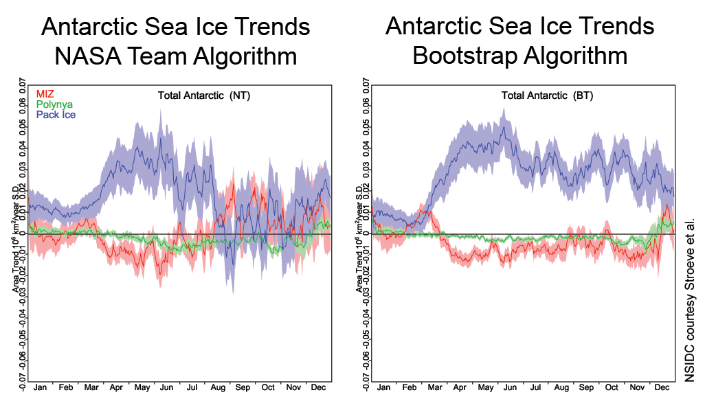
Throughout August, Arctic sea ice extent continued to track two or more standard deviations below the long-term average. The month saw two very strong storms enter the central Arctic Ocean from along the Siberian coast. In the Antarctic, ice extent remained near average.

Overview of conditions

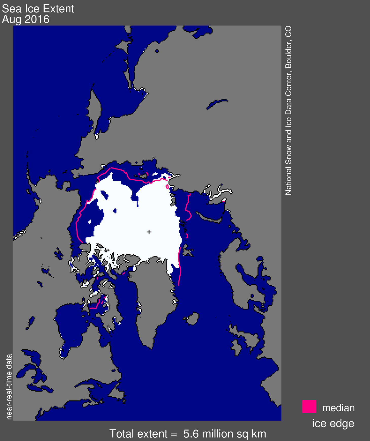
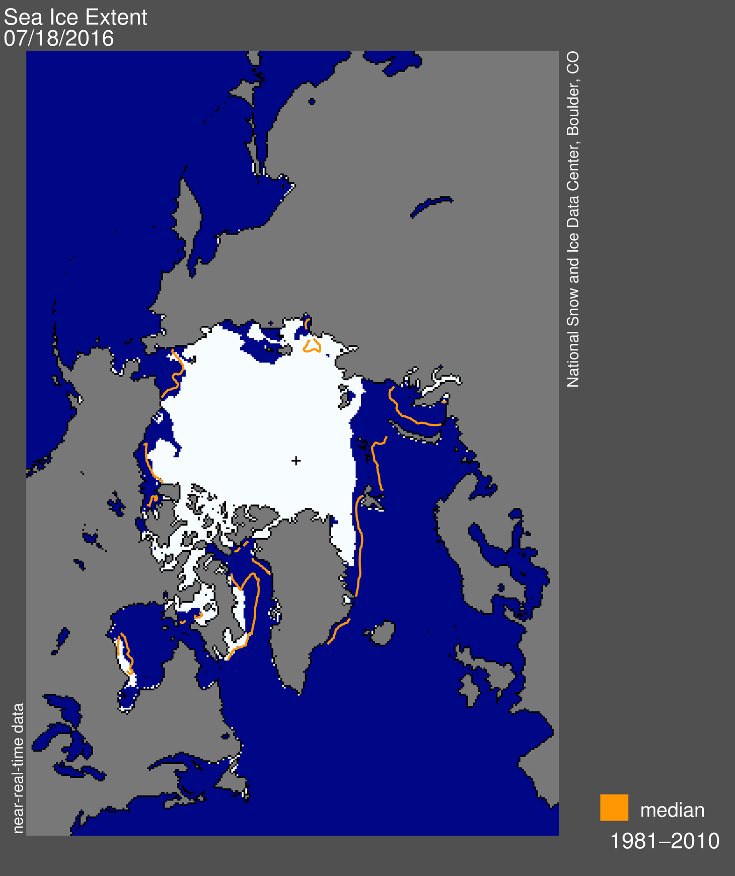
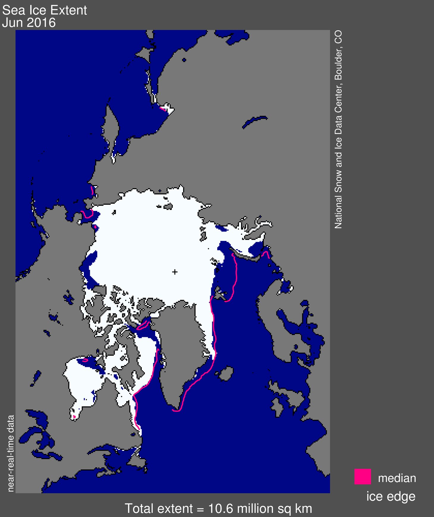
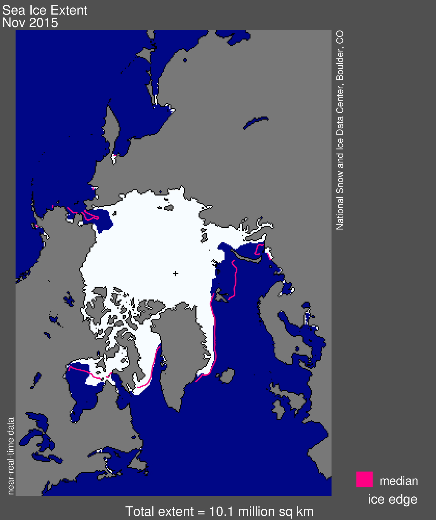
Figure 1. Arctic sea ice extent for August 2016 was 5.60 million square kilometers (2.16 million square miles). The magenta line shows the 1981 to 2010 median extent for that month. The black cross indicates the geographic North Pole. Sea Ice Index data. About the data

Credit: National Snow and Ice Data Center
High-resolution image

Average sea ice extent for August 2016 was 5.60 million square kilometers (2.16 million square miles), the fourth lowest August extent in the satellite record. This is 1.03 million square kilometers below the 1981 to 2010 average for the month and 890,000 square kilometers (344,000 square miles) above the record low for August set in 2012. As of September 5, sea ice extent remains below average everywhere except for a small area within the Laptev Sea. Ice extent is especially low in the Beaufort Sea and in the East Siberian Sea. With about two weeks of seasonal melt yet to go, it is unlikely that a new record low will be reached. However, since August 26, total sea ice extent is already lower than at the same time in 2007 and is currently tracking as the second lowest daily extent on record. In addition, during the first five days of September the ice cover has retreated an additional 288,000 square kilometers (111,000 square miles) as the tongue of sea ice in the Chukchi Sea has started to disintegrate.

Conditions in context

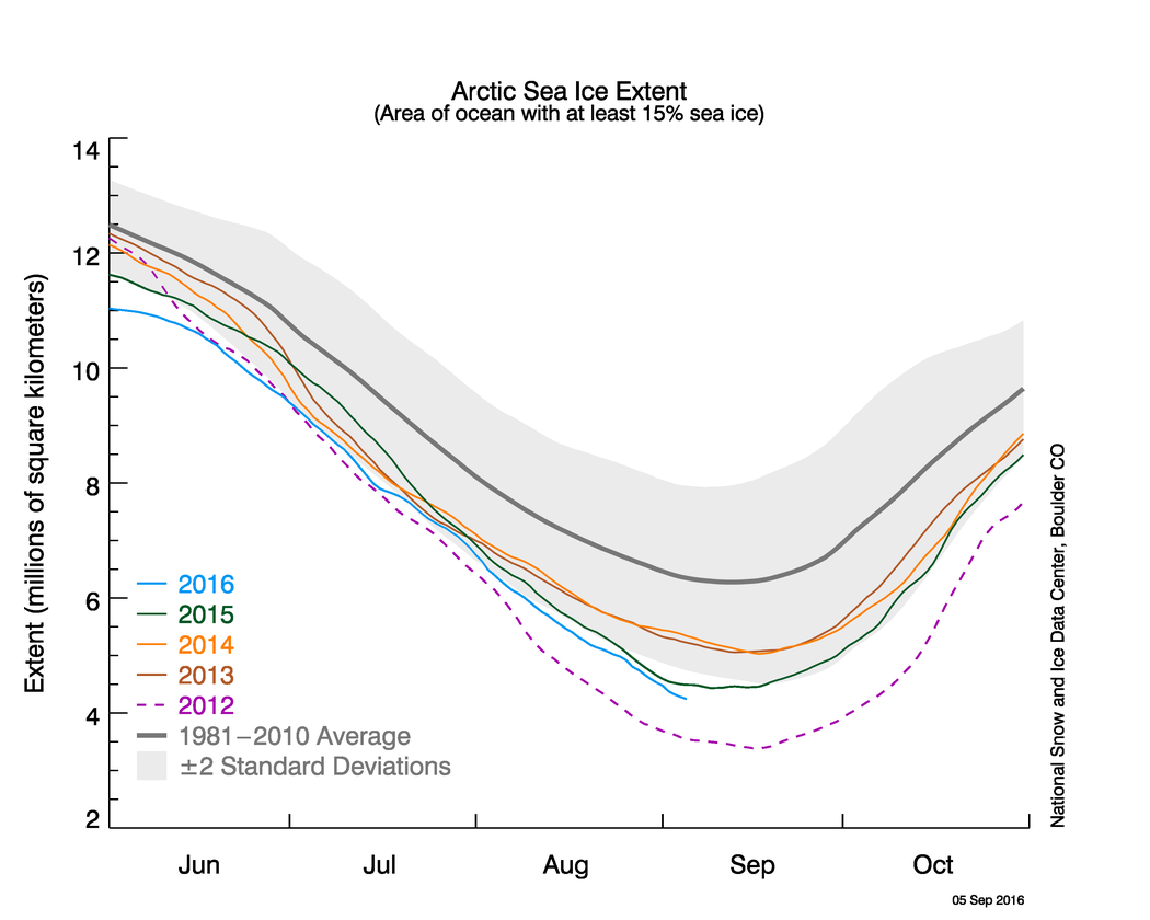
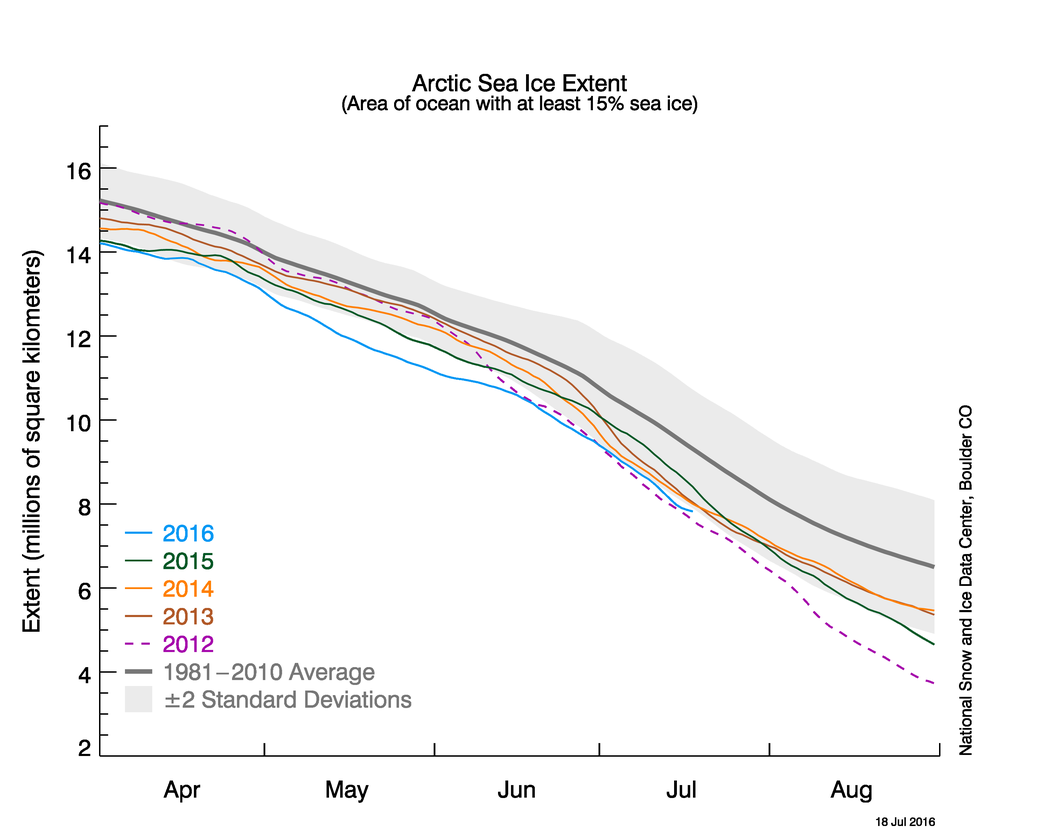
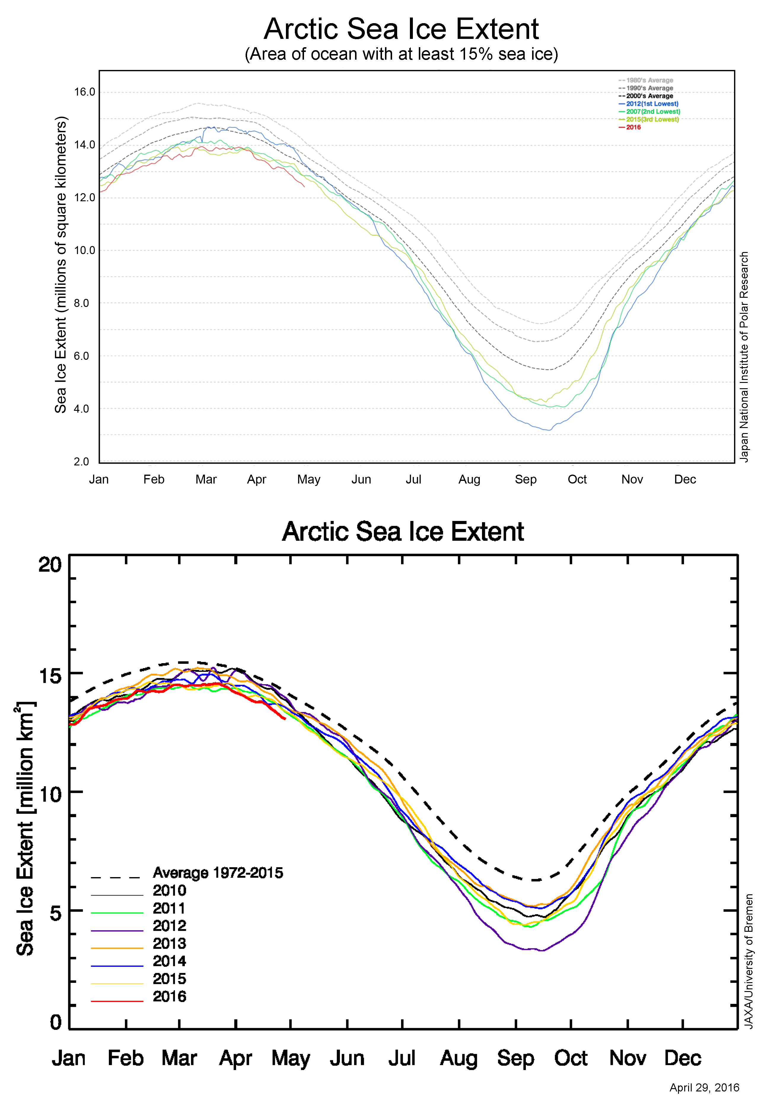
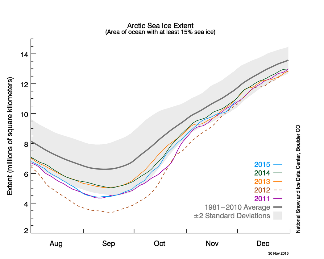
Figure 2a. The graph above shows Arctic sea ice extent as of September 5, 2016, along with daily ice extent data for four previous years. 2016 is shown in blue, 2015 in green, 2014 in orange, 2013 in brown, and 2012 in purple. The 1981 to 2010 average is in dark gray. The gray area around the average line shows the two standard deviation range of the data. Sea Ice Index data.

Credit: National Snow and Ice Data Center
High-resolution image

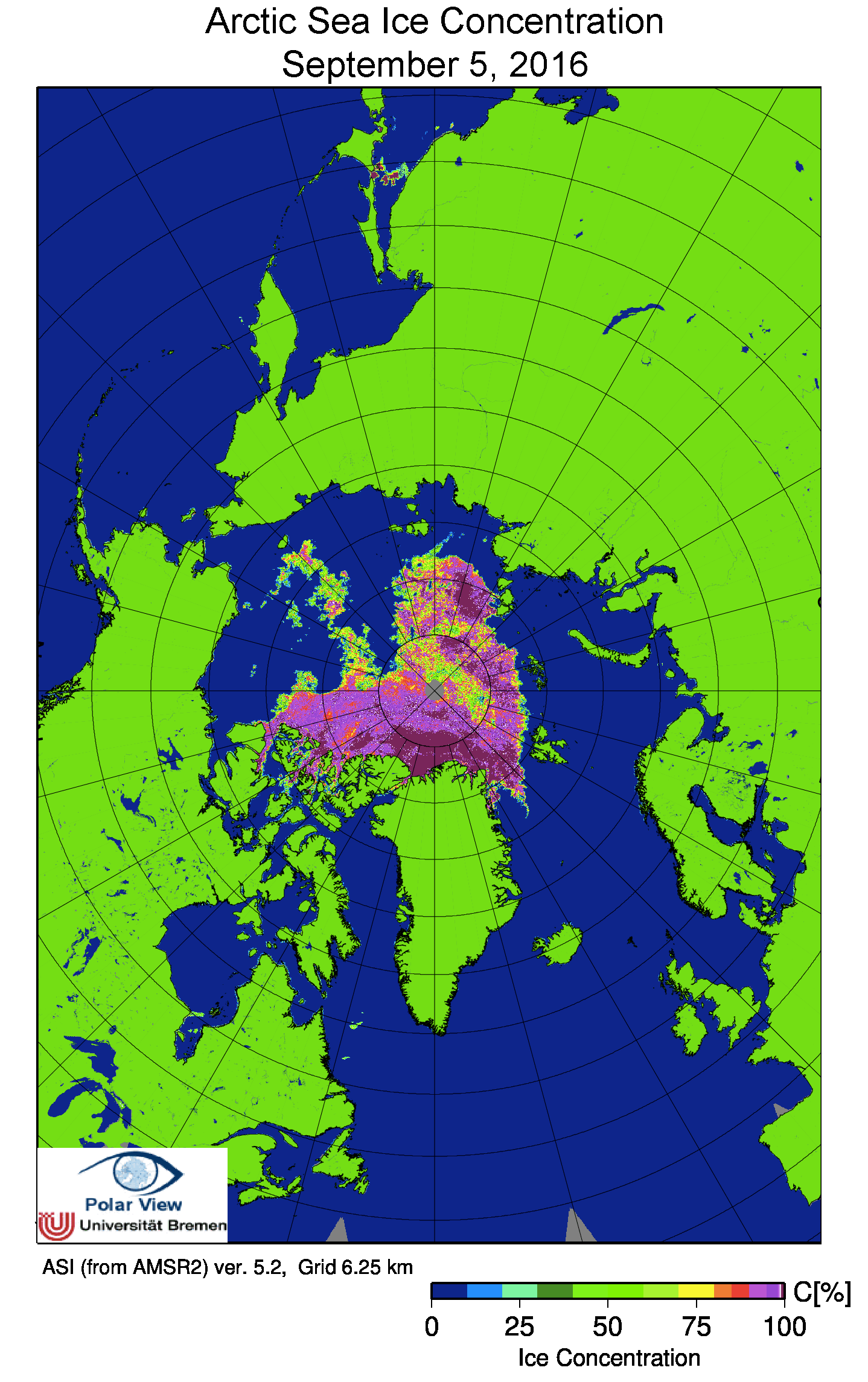
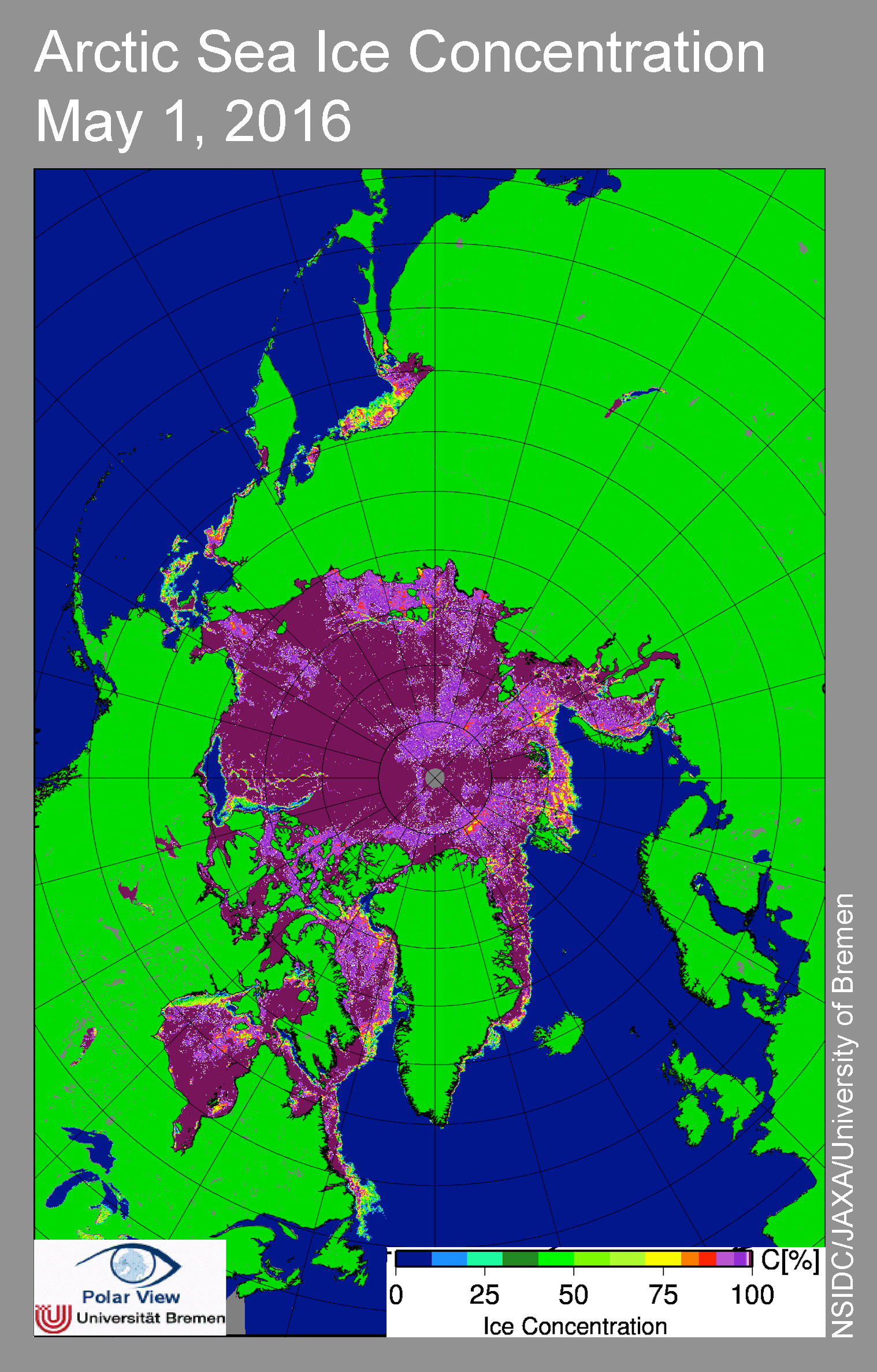
Figure 2b. The map shows Arctic sea ice concentration from the AMSR2 satellite instrument for September 5, 2016. Light blues and greens in ocean areas indicate areas of low ice concentration. The grey circle at the North Pole indicates where the satellite does not collect data, due to its orbit.

Credit: National Snow and Ice Data Center/University of Bremen
High-resolution image

The average ice loss rate through August was 75,000 square kilometers per day (29,000 square miles), compared to the long-term 1981 to 2010 average of 57,300 square kilometers per day (22,100 square miles per day), and a rate of 89,500 square kilometers per day for 2012 (34,500 square miles per day). Total ice extent loss in August was 2.34 million square kilometers (904,000 square miles).

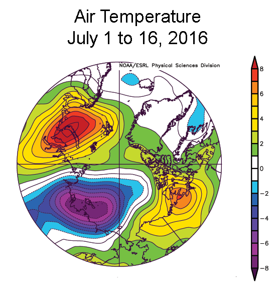
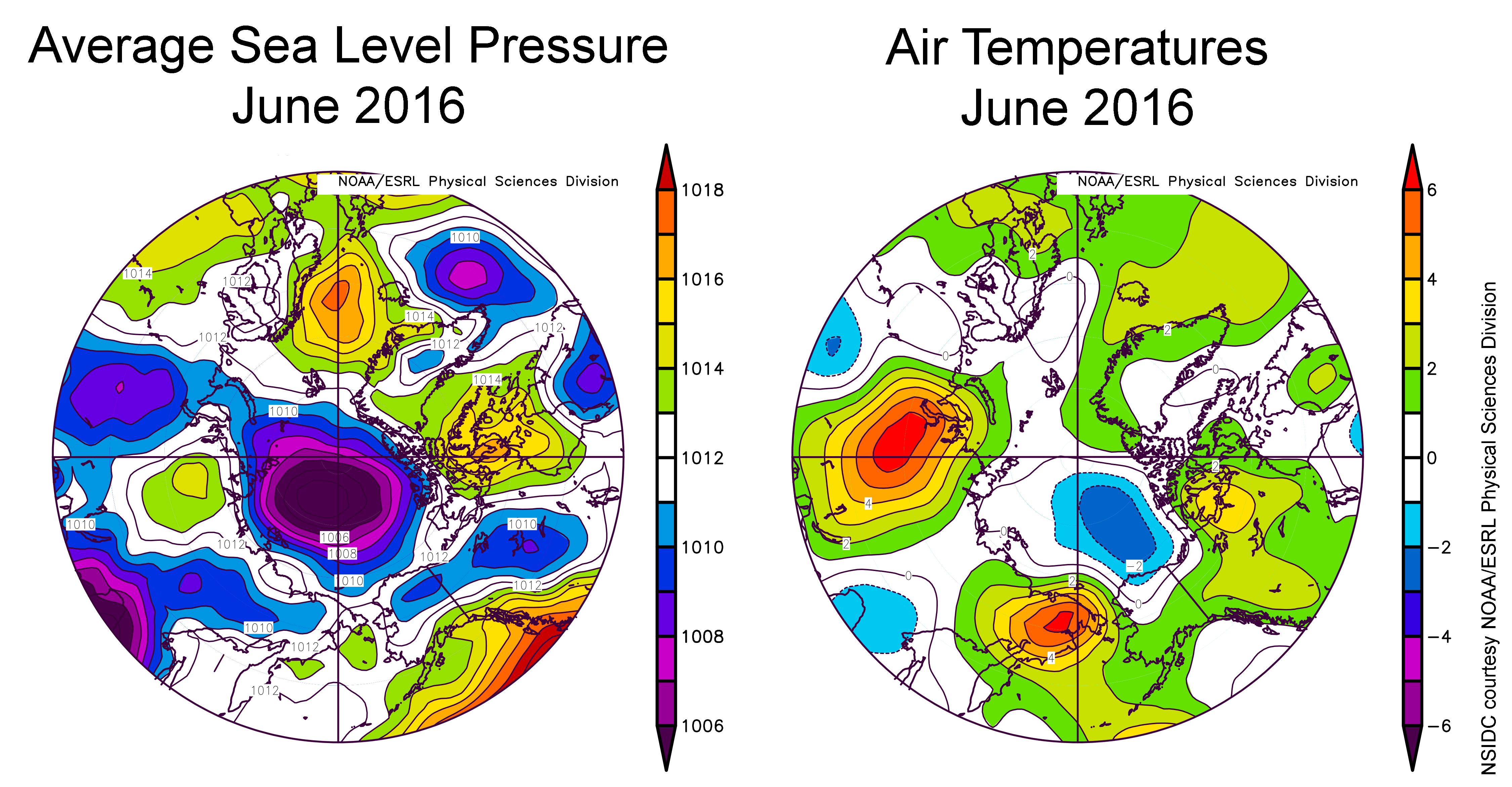
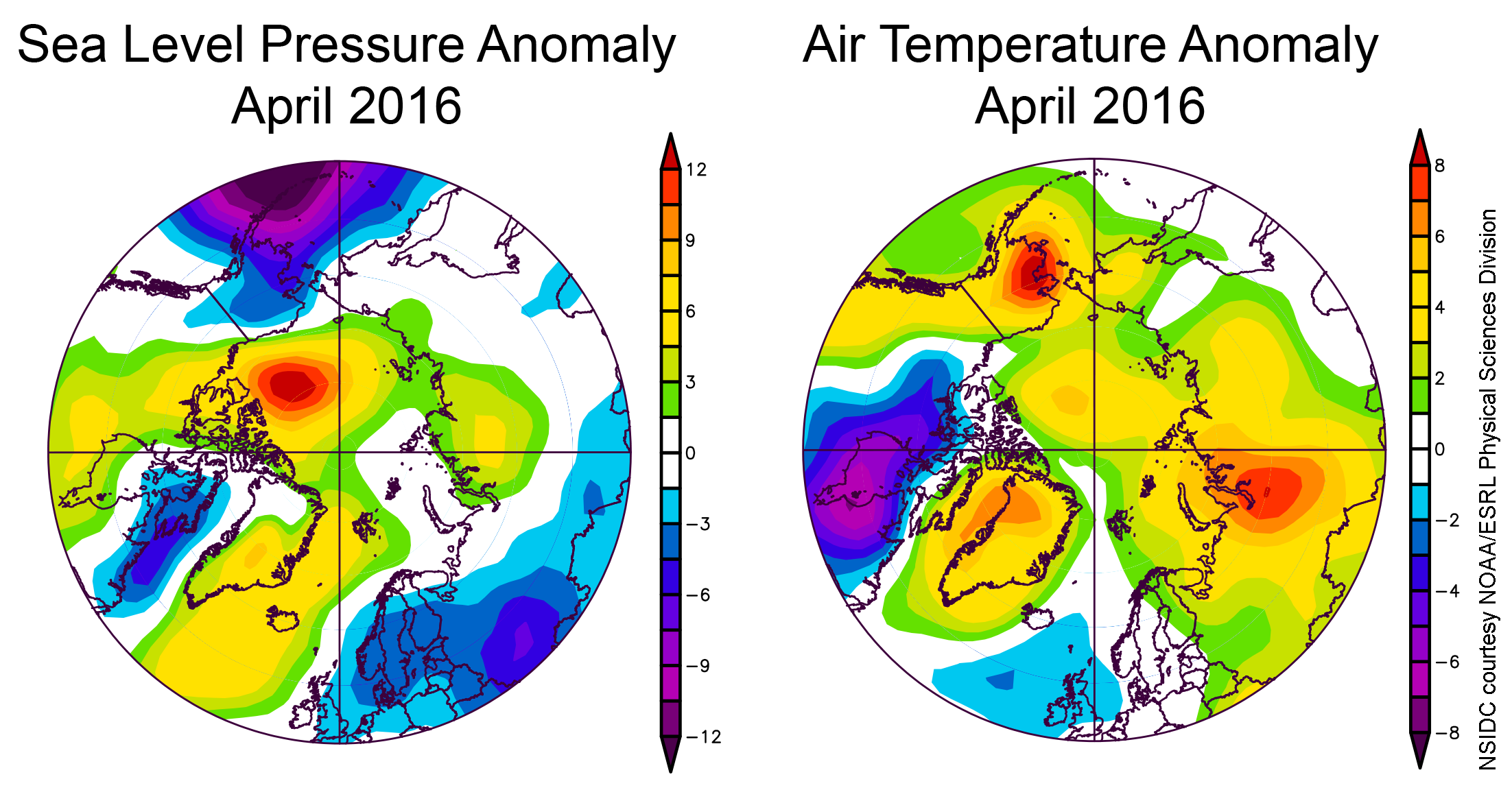
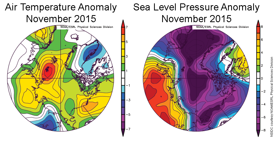
Air temperatures at the 925 hPa level were 1 to 3 degrees Celsius (2 to 5 degrees Fahrenheit) below average for a large area stretching from the northern Kara Sea, through the Laptev Sea, and into north-central Eurasia. Temperatures elsewhere over the Arctic Ocean were near average. Reflecting the generally stormy pattern through the month, sea level pressures were well below average (as much as 10 hPa) over the central and eastern Arctic Ocean. Two very strong cyclones entered the central Arctic Ocean in August from along the Siberian coast, bringing strong winds. On August 16, the central pressure of the first cyclone dropped to 968 hPa, nearly rivaling the storm in early August 2012 that attained a minimum central pressure of 966 hPa. On 22 August, the second storm started moving to the central Arctic Ocean along a similar track, and on August 23, attained a central pressure of 970 hPa.

Past studies have shown that stormy summers tend to end up with more sea ice at the end of the melt season than summers with high pressure over the central Arctic Ocean, primarily because stormy summers are both fairly cool and the wind pattern tends to spread the ice out. However, the impact of strong individual storms may be different—the 2012 event appears to have temporarily boosted ice loss by breaking up the ice cover, with the wave action tending to mix warmer waters from below to hasten melt. It may also be that, as the ice cover thins, its response to storms is changing.

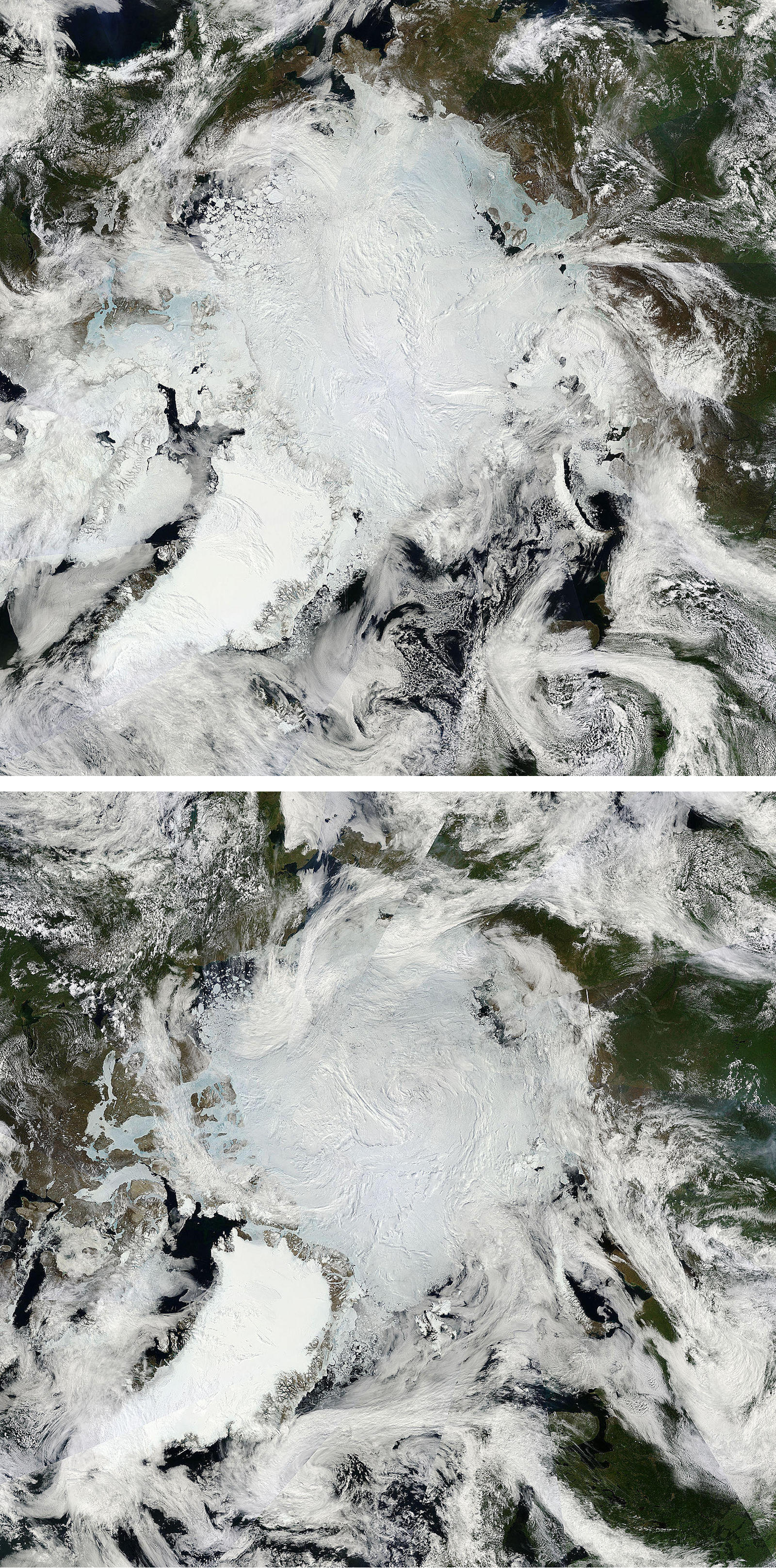
It indeed appears that the August 2016 storms helped to break up the ice and spread it out, contributing to the development of several large embayments and polynyas. Some of this ice divergence likely led to fragmented ice being transported into warmer ocean waters, hastening melt. Whether warmer waters from below were mixed upwards to hasten melt remains to be determined, but as discussed below, these storms were associated with very high wave heights.

August 2016 compared to previous years

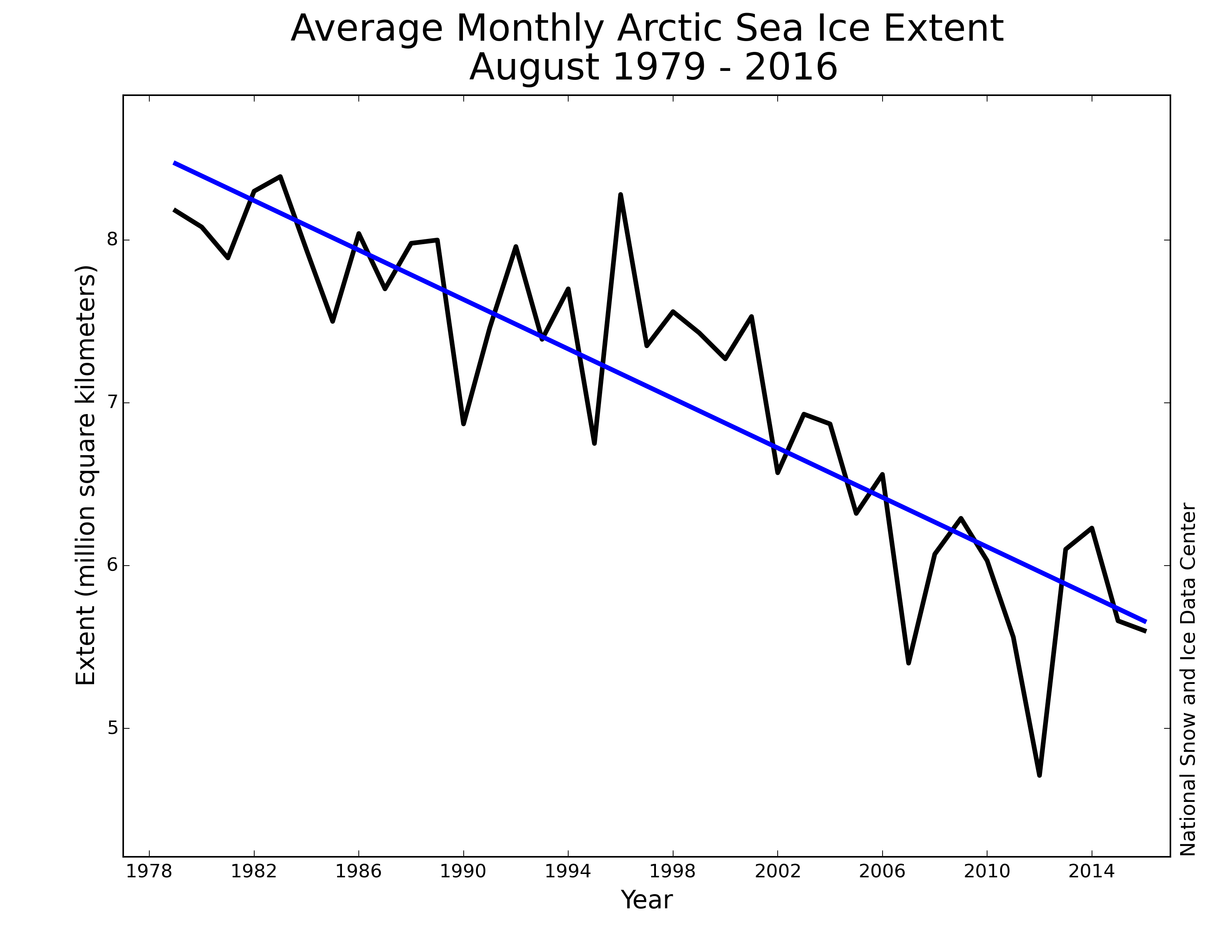
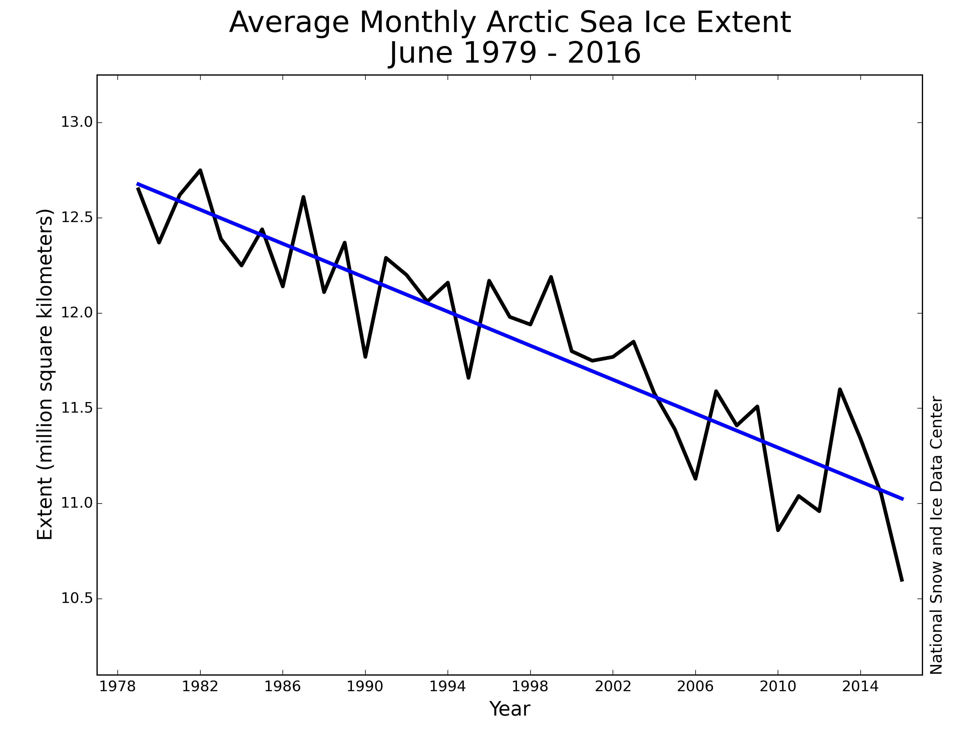
Figure 3. Monthly August ice extent for 1979 to 2016 shows a decline of 10.4 percent per decade.

Credit: National Snow and Ice Data Center
High-resolution image

Arctic sea ice extent averaged for August 2016 was the fourth lowest in the satellite data record. Through 2016, the linear rate of decline for August is 10.4 percent per decade.

Cyclones, ocean wave heights, and ice retreat

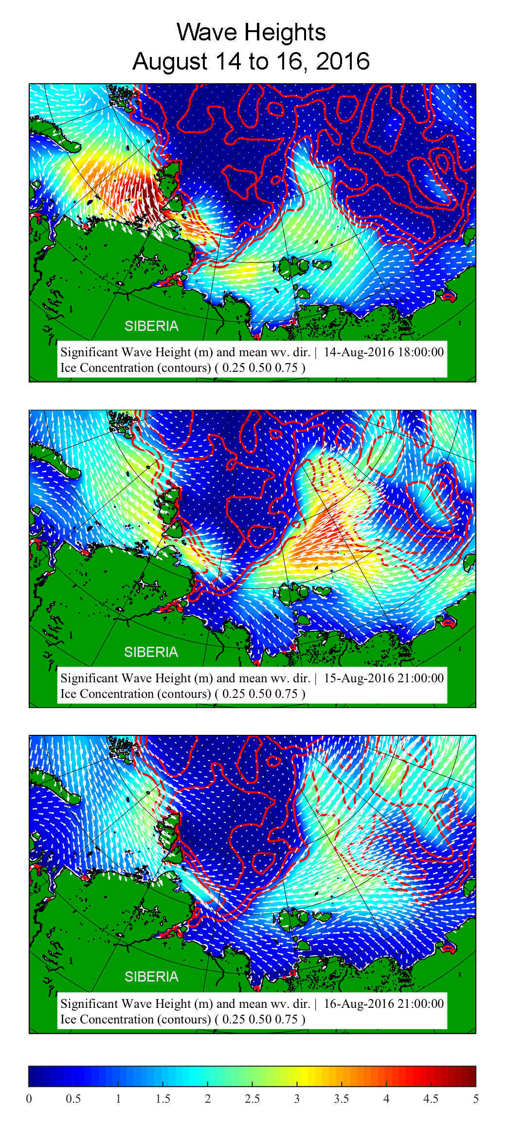
Figure 4. This series of plots shows significant wave height (in meters, indicated by color scale) in the western Arctic Ocean during the 2016 Arctic cyclone, from August 14 to August 16, 2016, as predicted by a numerical wave model (WAVEWATCH III), run at the Naval Research Laboratory (NRL). The solid red lines correspond to the analysis ice concentrations (25 percent, 50 percent and 75 percent) used as input for the wave model. White arrows indicate wave direction. This hindcast uses two time-varying inputs: 10-meter wind vectors from the atmospheric model NAVGEM (Navy Global Environmental Model, Hogan et al. 2014) run at the Fleet Numerical Meteorology and Oceanography Center (FNMOC), and analyses of ice concentrations (also produced at FNMOC) from passive microwave radiometer data (SSM/I). The wave model is run on a polar stereographic grid with a resolution of approximately 18 kilometers.

Credit: Erick Rogers, Naval Research Laboratory
High-resolution image

Large waves are common at high latitudes; 10-meter wave heights (33 feet) are not unusual for the Nordic Seas, and 15-meter wave heights (49 feet) can occur in the high latitudes of the Southern Ocean. However, large waves are a relatively new feature of the western Arctic Ocean. The height of waves is in part determined by surface wind speed, as well as the fetch (distance over open water that the wind can travel) and the duration of a wind event. A moderate sea ice cover damps ocean waves by absorbing and dispersing the wave energy through jostling of the ice floes against one another. A dense ice pack cover acts as a shield between the ocean and the surface wind, preventing wave formation.

In the latter half of the twentieth century, 4 to 6 meter waves (13 to 20 feet) rarely occurred in the western Arctic Ocean, but with more open water they have become more frequent, especially when strong storms enter the Arctic Ocean in late summer or early autumn. During the first of the two August cyclones discussed above, waves up to 5.9 meters (19 feet) were predicted. This occurred during the early part of the cyclone’s lifecycle (1800 UTC August 14), in the eastern Kara Sea. Further east, north of the New Siberian Islands, wave heights were estimated as high as 4.3 meters (14 feet) late on August 15. In this region, the waves were directly incident on the ice edge. In response, the ice edge retreated following the 4.3 meter waves on August 15.

Northwest Passage update

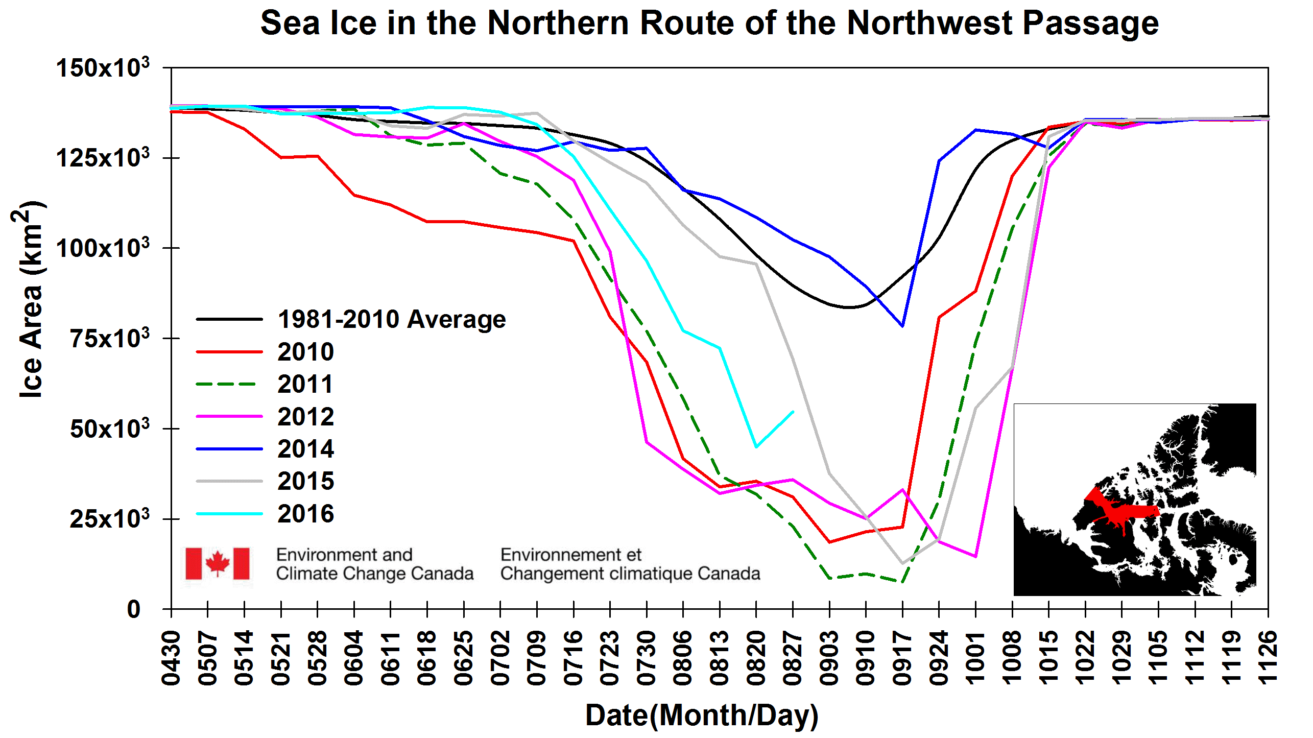
Figure 5. The time series shows total sea ice area for selected years and the 1981-2010 average within the northern route of the Northwest Passage. The cyan line shows 2016 and other colors show ice conditions in different years. Data are from the Canadian Ice Service.

Credit: Stephen Howell, Environment and Climate Change Canada
High-resolution image

The Northwest Passage refers to the fabled shortcut between the Atlantic and Pacific through the Canadian Archipelago. However, it is not one route. There is a northern, deep-water route through the Parry Channel, entered from the west through the M’Clure Strait and a shallower southern route, known as Amundsen’s route. Sea ice in the Parry Channel route has shown a sharp decline since the middle of July, but the channel is still not entirely ice free. Considerable ice remains in the western (M’Clure Strait) region and there are lesser amounts in the eastern regions. This is mostly (~80 percent) multiyear ice. Low ice years in the Parry Channel are typically the result of early summer breakup associated with high sea level pressure over the Beaufort Sea and Canada Basin that displace the Arctic Ocean pack ice away from the western entrance. Conversely, low sea level pressure anomalies over the Beaufort Sea and Canada Basin keep the Arctic Ocean pack ice up against the western entrance. This has been the case for much of the 2016 melt season. The southern (Amundsen’s) route is open but it is still uncertain whether the northern route will open in the coming weeks.

Even during mild ice years, thick multiyear ice is typically advected into these routes during the summer months. Multiyear ice is a significant obstacle for ships. Nevertheless, taking advantage of mild sea ice conditions, the 68,000-ton Crystal Serenity set sail from Anchorage, Alaska on August 16 for its 32-day journey through the Northwest Passage via Amundsen’s route. This is the largest ship thus far to navigate the Northwest Passage and is accompanied by an icebreaker ship and two helicopters. The ship sailed through the Northwest Passage in less than three weeks—52 times faster than Amundsen’s nearly three-year voyage.

On the other side of the Arctic, the Northern Sea Route appears mostly ice free.

Further reading

Collins, C. O., W. E. Rogers, A. Marchenko and A. V. Babanin. 2015. In situ measurements of an energetic wave event in the Arctic marginal ice zone. Geophysical Research Letters, 42, doi:10.1002/2015GL063063.

Haas, C., and S. E. L. Howell. 2015. Ice thickness in the Northwest Passage. Geophysical Research Letters, 42, 7673–7680, doi:10.1002/2015GL065704.

Hogan, T., et al. 2014. The Navy Global Environmental Model, Oceanography, 27(3), 116-125.

Howell, S. E. L., T. Wohlleben, M. Dabboor, C. Derksen, A. Komarov and L. Pizzolato. 2013. Recent changes in the exchange of sea ice between the Arctic Ocean and the Canadian Arctic Archipelago. Journal of Geophysical Research, 118, 3595–3607, doi:10.1002/jgrc.20265.

Thomson, J., and W. E. Rogers. 2014. Swell and sea in the emerging Arctic Ocean, Geophysical Research Letters 41, doi:10.1002/2014GL059983.

Thomson, J. et al. 2016. Emerging trends in the sea state of the Beaufort and Chukchi seas, Ocean Modelling 105, doi:10.1016/j.ocemod.2016.02.009.

Through the first half of July, Arctic sea ice extent continued tracking close to levels in 2012, the summer that ended with the lowest September extent in the satellite record. The stormy weather pattern that characterized June has persisted into July. Nevertheless, sea ice melt began earlier than average over most of the Arctic Ocean.

Overview of conditions

Figure 1. Arctic sea ice extent for July 18, 2016 was 7.82 million square kilometers (3.02 million square miles). The orange line shows the 1981 to 2010 median extent for that day. The black cross indicates the geographic North Pole. Sea Ice Index data. About the data

Credit: National Snow and Ice Data Center
High-resolution image

As of July 18, Arctic sea ice extent was 7.82 million square kilometers (3.02 million square miles). This is just below the two standard deviation value for the date, and just above the level observed on the same date in 2012, the year that ended up having the lowest September extent in the satellite record. Throughout the month, extent has closely tracked both the two standard deviation and 2012 levels.

Ice extent in the first half of July was well below average in the Kara and Barents seas, as it has been throughout the winter and spring. Extent is also below average in the Beaufort and Chukchi seas, between the East Siberian and Laptev seas by the New Siberian Islands, and along the southeast coast of Greenland. In the last several days, polynyas have formed in the northern Beaufort Sea. Compared to 2012 at this time of year, there is more ice in the southern Beaufort Sea, Baffin Bay, the Laptev Sea, and north of the New Siberian islands in the East Siberian Sea. There is less ice this year in the East Greenland Sea, extending through the Barents and Kara seas, and in the western Beaufort and Chukchi seas.

Conditions in context

Figure 2. The graph above shows Arctic sea ice extent as of July 18, 2016, along with daily ice extent data for four previous years. 2016 is shown in blue, 2015 in green, 2014 in orange, 2013 in brown, and 2012 in purple. The 1981 to 2010 average is in dark gray. The gray area around the average line shows the two standard deviation range of the data. Sea Ice Index data.

Credit: National Snow and Ice Data Center
High-resolution image

Figure 3. This surface weather map from the Canadian Meteorological Center for 0600Z, July 6, 2016, shows a strong low pressure system (extratropical cyclone) over the Eurasian side of the central Arctic Ocean. The central pressure of the cyclone dropped to as low as 979 hPa, a very strong storm for this part of the Arctic.

Credit: National Snow and Ice Data Center/Canadian Meteorological Center
High-resolution image

Figure 4. Arctic air temperatures at the 925 hPa level, as compared to the long-term (1981 to 2010) average. The area of below average temperatures centered over the East Siberian Sea contrasts sharply with unusually warm conditions over the Barents and Kara seas, the Canadian Arctic Archipelago and northern Alaska.

Credit: NSIDC/ NOAA ESRL Physical Sciences Division
High-resolution image

The average rate of ice loss through July 18 was 89,500 square kilometers (34,600 square miles) per day, which is close to the long-term average (1981 through 2010) rate of 86,800 square kilometers (33,500 square miles) per day. Recall from our last post that the month of June was characterized by a stormy pattern over the central Arctic Ocean, which likely acted to slow the rate of ice loss. This pattern has persisted into July. However, the rate of decline increased in the first two weeks of the month as very warm conditions spread around the Arctic coasts. Ice loss has slowed in the last few days. A number of low pressure systems, primarily generated over northern Eurasia, have migrated into the central Arctic Ocean, north of the East Siberian Sea. One of these was quite strong, with a central pressure dropping to as low as 979 hPa (Figure 3).

Cyclones found over the central Arctic Ocean in summer tend to be what is termed “cold cored.” Because of these cold-cored systems and their associated pattern of winds, air temperatures at the 925 hPa level for the first half of July have been well below average along and north of the East Siberian Sea. By sharp contrast, strongly above average temperatures have been the rule over the Barents and Kara seas, the Canadian Arctic Archipelago and northern Alaska (Figure 4). Local conditions can be quite variable, and not well captured by conditions at the 925 hPa level. On July 14, Deadhorse, on the North Slope of Alaska on the shores of the Beaufort Sea, saw a record high temperature. The reading of 85° Fahrenheit (through 7 p.m.) broke the record of 83° Fahrenheit set in 1991. It is also also the highest reading on record for any Alaska station within 50 miles of the Arctic Ocean coast north of the Brooks Range.

Early melt onset

Figure 5. The onset of surface melt, as determined from satellite passive microwave data, was early over most of the Arctic Ocean. An early melt implies an early drop in the surface albedo, which furthers the melt process.

Credit: National Snow and Ice Data Center
High-resolution image

Seasonal onset of surface melt was early over most of the Arctic Ocean (Figure 5). This occurred under the high-pressure-dominated weather pattern that was present earlier in the spring. The onset of surface melt can be determined with the same passive microwave data used to determine sea ice extent and concentration. Melt began in late April/early May in the southern Beaufort Sea, which was about 6 weeks (more than 40 days) earlier than average. Melt also began a month earlier than average in the Barents Sea and northern Baffin Bay.

Early onset of melt is important because melt drops the surface albedo, allowing the sea ice and its overlying snow cover to absorb more solar radiation, which accelerates the melt process. Data from the NASA Moderate Resolution Imaging Spectroradiometer (MODIS) satellite instrument show many very large, multiyear ice floes in the Beaufort Sea, one of them about 50 miles across. It will be interesting to see if these large multiyear floes melt out this summer. NSIDC will be closely monitoring the situation.

New insights into Antarctic sea ice conditions

Gerald Meehl of the National Center for Atmospheric Research led a new study shedding light on the upward trend in total Antarctic sea ice extent over the period of satellite observations. The overall view from climate models is that Antarctic sea ice extent should have decreased in response to the general warming of climate. This has led some scientists to suggest that the climate models are fundamentally flawed. However, an explanation for the expanding Antarctic sea ice appears to lie in the Interdecadal Pacific Oscillation (IPO), a natural mode of climate variability. The IPO transitioned from a positive to a negative phase in the late 1990s at the same time that the increase in total Antarctic sea ice extent accelerated. The negative IPO brought a cooling of tropical Pacific sea surface temperatures, and deepening of the Amundsen Sea Low near Antarctica. This has contributed to regional circulation changes in the Ross Sea region favoring expansion of the sea ice cover. Meehl’s study also shows that the negative phase of the IPO in coupled global climate models is characterized by patterns similar to the sea-level pressure and 850 hPa wind changes observed in all seasons near Antarctica since 2000, particularly in the Ross Sea region. Additional model experiments show that these atmospheric circulation changes are mainly driven by precipitation and convective heating anomalies related to the IPO in the equatorial eastern Pacific. They conclude that the models are not wrong, but instead can simulate the processes involved with natural climate variability that results in increased Antarctic sea ice, even when global temperatures are rising.

Reference

Meehl, G.A., J.M. Arblaster, C. Bitz, C.T.Y. Chung, and H. Teng. 2016. Antarctic sea ice expansion between 2000-2014 driven by tropical Pacific decadal climate variability. Nature Geoscience, doi:10.1038/NGEO2751.

June set another satellite-era record low for average sea ice extent, despite slower than average rates of ice loss. The slow rate of ice loss reflects the prevailing atmospheric pattern, with low pressure centered over the central Arctic Ocean and lower than average temperatures over the Beaufort Sea.

Overview of conditions

Figure 1. Arctic sea ice extent for June 2016 was 10.60 million square kilometers (4.09 million square miles). The magenta line shows the 1981 to 2010 median extent for that month. The black cross indicates the geographic North Pole. Sea Ice Index data. About the data

Credit: National Snow and Ice Data Center
High-resolution image

Arctic sea ice extent during June 2016 averaged 10.60 million square kilometers (4.09 million square miles), the lowest in the satellite record for the month. So far, March is the only month in 2016 that has not set a new record low for Arctic-wide sea ice extent (March 2016 was second lowest, just above 2015). June extent was 260,000 square kilometers (100,000 square miles) below the previous record set in 2010, and 1.36 million square kilometers (525,000 square miles) below the 1981 to 2010 long-term average.

Sea ice extent remains below average in the Kara and Barents seas, as it has throughout the winter and spring. Despite lower than average temperatures over the Beaufort Sea, sea ice extent there remains below average, and was the second lowest extent for the month of June during the satellite data record.

Conditions in context

Figure 2a. The graph above shows Arctic sea ice extent as of July 5, 2016, along with daily ice extent data for four previous years. 2016 is shown in blue, 2015 in green, 2014 in orange, 2013 in brown, and 2012 in purple. The 1981 to 2010 average is in dark gray. The gray area around the average line shows the two standard deviation range of the data. Sea Ice Index data.

Credit: National Snow and Ice Data Center
High-resolution image

Figure 2b. The map of sea level pressure averaged for the month of June 2016 (left) shows low pressure over the central Arctic Ocean. The map of air temperatures at 925 hPa for June 2016 compared to the 1981 to 2010 long-term average (right) shows cool conditions over the Beaufort Sea.

Credit: NSIDC courtesy NOAA/ESRL Physical Sciences Division
High-resolution image

The average rate of ice loss during June 2016 was 56,900 square kilometers (22,000 square miles) per day, but was marked by two distinct regimes. First, there was a period of slow loss during June 4 to 14 of only 37,000 square kilometers (14,000 square miles) per day. This was followed by above average rates (74,000 square kilometers, or 29,000 square miles) for the rest of the month. For the month as a whole, the rate of loss was close to average (53,600 square kilometers per day). The slow ice loss during early June was a result of a significant change in the atmospheric circulation. May was characterized by high surface pressure over the Arctic Ocean, a basic pattern that has held since the beginning of the year. However, June saw a marked shift to low pressure over the central Arctic Ocean. This type of pattern is known to inhibit ice loss. A low pressure pattern is associated with more cloud cover, limiting the input of solar energy to the surface, as well as generally below average air temperatures. However, in June 2016, it was only in the Beaufort Sea where air temperatures at the 925 hPa level were distinctly below average (about 2 degrees Celsius below average, or 4 degrees Fahrenheit). The change in circulation also shifted the pattern of ice motion. In general, winds associated with such a low pressure pattern will tend to spread the ice out (that is, cause the ice to diverge).

June 2016 compared to previous years

Figure 3. Monthly June ice extent for 1979 to 2016 shows a decline of 3.7% per decade.

Credit: National Snow and Ice Data Center
High-resolution image

Through 2016, the rate of decline for the month of June is 44,600 square kilometers (17,200 square miles) per year, or 3.7 percent per decade. June extent remained below 2012 levels throughout the month, but it was above the 2010 extent for several days. 2010 had the lowest extent for several days during June.

View from above

Figure 4. MODIS composite images for June 9, 2016 (top) and June 28, 2016 (bottom) show the seasonal progression of surface melting and darkening of the ice surface.

Credit: Land Atmosphere Near-Real Time Capability for EOS (LANCE) System, NASA/GSFC
High-resolution image

The Moderate Resolution Imaging Spectroradiometer (MODIS) instruments on the NASA Aqua and Terra satellites provide multiple views each day of the Arctic, and in summer the entire region is sunlit. Two mosaics for June 9 and June 28 show the seasonal progression in surface melting and darkening of the sea ice; the blue-green areas where surface ponding is present; and the movement of large sea ice floes in the Beaufort Sea. On June 9, the ponds are most evident in the Laptev Sea off the coast of Siberia; on June 28, the ponds are most evident in the Canadian Archipelago.

A quick look at sea ice thickness fields

Figure 5. Sea ice thickness from April and May 2016 from Operation IceBridge. Image courtesy Nathan Kurtz, NASA Goddard.

Credit: N. Kurtz, NASA Goddard Space Flight Center
High-resolution image

Results from NASA’s Operation IceBridge aircraft missions conducted during late April and early May indicate that ice thicknesses from the Alaskan coast of the Beaufort Sea up to the North Pole were generally in the 2 to 3 meter range (7 to 10 feet), indicative of multiyear ice. However, substantial variations were found along the flight transects with several locations showing an ice thickness of 1.5 meters (5 feet) or less, indicative of first-year ice, while in other locations thicknesses were over 5 meters (16 feet), corresponding to either fairly thick multiyear ice or ridged first-year ice. This substantial variation is representative of a broken up and variegated ice pack with thick multiyear floes interspersed with thinner first-year ice.

The first-year thicknesses were found to be generally thinner than is typical at the end of winter, which is consistent with the usually high temperatures characterizing last winter. Very thin ice (less than 0.5 meters, or 1.6 feet) was found in places near the Alaskan coast, where leads opened up fairly late in the ice growth season. The IceBridge results are generally in agreement with the ice thickness surveys conducted in early April by researchers from York University, and with CryoSat-2 thickness maps discussed in our previous post.

Sea Ice Outlook

Each summer the Sea Ice Prediction Network (SIPN) requests forecasts of the September average sea ice extent. Requests are made in June July and August. This year, thirty contributions to the June Sea Ice Outlook were received, employing a variety of methods, including statistical models, dynamical models, and informal polls. The median prediction for this year’s September sea ice extent is 4.28 million square kilometers (1.65 million square miles), similar to the extent observed in 2007. Dynamical models predict 4.58 million square kilometers (1.77 million square miles), compared to the slightly lower overall median extent prediction of 4.28 million square kilometers (1.65 million square miles) from statistical models. The lowest median extent comes from the heuristic contributions (4.0 million square kilometers, or 1.5 million square miles). Only one forecast points towards a new record low for 2016.

Antarctic sea ice

Figure 6. Circumpolar Antarctic trends from 1979 to 2014 in the consolidated pack ice (blue), the marginal ice zone (red) and coastal polynyas (green) from the NASA Team sea ice algorithm (left) and the Bootstrap algorithm (right).

Credit: National Snow and Ice Data Center, Stroeve et al.
High-resolution image

Antarctic sea ice extent continues to track at near average levels, in sharp contrast to the previous two winters, which were above average. While the total ice extent in the Antarctic shows a small positive trend, particularly during the cold season, whether or not the total mass of the ice has changed depends on how much of the pack ice consists of consolidated ice, the extent of the marginal ice zone (the outer edge of the ice pack, which is lower in ice concentration), and coastal polynyas (open water areas near the coast). The marginal sea ice zone and the coastal polynyas have important biological implications. These are key regions for phytoplankton productivity and krill abundance that in turn feed Antarctic sea birds and nektonic fauna (things that swim).

A new study looks at how these regions are changing using two sea ice concentration algorithms distributed by NSIDC. While the algorithms give similar trends in the overall sea ice extent, they differ in terms of whether or not the sea ice cover is becoming more compacted (i.e., the consolidated ice pack is increasing in extent) or if the marginal ice zone is expanding (Figure 6). When sea ice is is growing seasonally, both algorithms indicate that it is due to an expansion of the consolidated ice pack, whereas during winter and spring, one measurement method (the NASA Team algorithm) finds the marginal ice zone is also expanding as well, and the other measurement (Bootstrap algorithm) shows no significant trend in the marginal ice. The algorithms also differ in how much of the total ice pack consists of pack ice or the marginal ice, with the NASA Team algorithm having on average twice as large of a marginal ice zone as the Bootstrap algorithm. As well, the NASA Team algorithm is known to underestimate ice concentration in the Antarctic. This highlights the need for further validation of sea ice concentrations derived from passive microwave satellite data.

New Sea Ice Index version

As part of our quality control process, the Sea Ice Index, which supplies sea ice extent and concentration values, has been updated to Version 2. Changes include using the most recently available version of the Sea Ice Concentrations from Nimbus-7 SMMR and DMSP SSM/I-SSMIS Passive Microwave Data that provide final sea ice concentration data. The version update also adjusted three procedures in the Sea Ice Index processing routine that affected both the near-real-time data and the final data. These four updates affect different portions of the Sea Ice Index time series. Because of these updates, minor changes in some of the ice extent and area numbers will be seen. However, these changes are almost all quite small and do not alter current conclusions about Arctic or Antarctic sea ice conditions. More information on Version 2 is available in the Sea Ice Index documentation.

Reference

Stroeve, J. C., Jenouvrier, S., Campbell, G. G., Barbraud, C., and Delord, K. 2016, in review. Mapping and assessing variability in the Antarctic Marginal Ice Zone, the pack ice and coastal polynyas. The Cryosphere Discuss., doi:10.5194/tc-2016-26.

As of June 14, 2016, NSIDC has completed the transition to the Defense Meteorological Satellite Program (DMSP) F-18 satellite for sea ice data. Sea Ice Index updates have also resumed.

Sea ice data in Arctic Sea Ice News and Analysis are now based on the F-18 satellite beginning April 1, 2016. Data before April 1 are still from the F-17 satellite or earlier satellites in the series.

For more information on the F-17 satellite issues, see our April 12, 2016 post. On May 6, updates resumed with provisional F-18 data. These data are no longer considered provisional. However, these are near-real-time data and numbers may change when final data are obtained.

For more information on the satellite transition, see the documentation for the Near-Real-Time DMSP SSMIS Daily Polar Gridded Sea Ice Concentrations data set.

NSIDC has obtained data from the DMSP F-18 satellite and is in the process of intercalibrating the F-18 data with F-17 data. Intercalibration addresses differences between the series of sensors, in order to provide a long-term, consistent sea ice record. While this work continues, we are displaying the uncalibrated F-18 data in the daily extent image. The daily time series graph shows F-17 data through March 31, and F-18 data from April 1 forward. Initial evaluation of the uncalibrated F-18 data indicates reasonable agreement with F-17, but the data should be considered provisional and quantitative comparisons with other data should not be done at this time.

Because these are provisional data, the Sea Ice Index has not been updated and continues to display only F-17 data through March 31. We expect to make the F-18 data available in Charctic soon.

For general information on the intercalibration of sensors, see the documentation for Sea Ice Concentrations from Nimbus-7 SMMR and DMSP SSM/I-SSMIS Passive Microwave Data. This documentation will be updated when the intercalibration to F-18 is complete.

For more information on the F-17 satellite sensor issues, see our previous post.

The Defense Meteorological Satellite Program (DMSP) F17 satellite is experiencing continuing issues with its passive microwave sensor. Data from the 37V channel, used to observe sea ice, have been unusable since early April, although the 37H channel used for the Greenland Ice Sheet Today melt area mapping is unaffected. NSIDC is working to bring the DMSP F18 satellite online for its near-real-time source of data for sea ice monitoring. Based on other data sources, sea ice extent remains far below average for the satellite record period, and likely setting record daily lows. The April sea ice decline rate appears to have been slightly faster than average.

Overview of conditions

Figure 1a. Arctic sea ice concentration, in percent concentration, for May 1, 2016 from the Japan Aerospace Exploration Agency (JAXA) satellite Shizuku (GCOM-W1) AMSR2 instrument. Areas of ocean with at least 15% ice concentration are considered ice-covered, when calculating sea ice extent.

Credit: Japan Aerospace Exploration Agency, courtesy University of Bremen
High-resolution image

Figure 1b. The graphs show Arctic sea ice extent as of April 29, 2016, along with ice extent data for previous years. Top, sea ice extent for 2016 from the Japan Aerospace Exploration Agency (JAXA) satellite Shizuku (GCOM-W1) AMSR2 instrument. Bottom, similar plot using the same sensor but a different method and channel, from University of Bremen.

Credit: National Snow and Ice Data Center/JAXA/University of Bremen
High-resolution image

The Arctic Sea Ice News and Analysis reference sea ice product, the Sea Ice Index, will be suspended until a new calibration can be completed for the F18 satellite, which is underway. The Advanced Microwave Scanning Radiometer 2 (AMSR2) instrument flying on Shizuku (GCOM-W1), a satellite operated by the Japan Aerospace Exploration Agency (JAXA), provides data on sea ice extent and rates of change, but because it uses a different sensor and processing algorithm, the extent numbers cannot be directly compared with those from the SMMR-SSM/I-SSMIS instruments record; the AMSR2 algorithm gives extents that differ by several tens of thousands of square kilometers, or a fraction of a percent to a few percent of total sea ice extent.

A look at the Arctic Data archive system at the National Institute of Polar Research in Japan reveals that sea ice since mid-April has remained at record low daily levels as assessed over their archive of sea ice extent, and is approximately 400,000 square kilometers (154,400 square miles) below the previous daily record extents at this time. This is supported by another analysis of sea ice extent produced by the University of Bremen using the same satellite but a different sensor channel. Both assessments of sea ice extent indicate that the April rate of decline for 2016 is slightly faster than the long-term average of their respective archives. Another sea ice monitoring site, The Cryosphere Today, continues to use the DMSP F17 data, and their graphics show evidence of the sensor issues. This site reports sea ice area in its graphical trend, not extent (area of ocean with at least 15% sea ice coverage) as do the other sites and NSIDC. However, the trend and record low daily extents for the second half of April may be interpreted from these data as well.

Conditions in context

Figure 2. Left, sea level pressure for April 2016 relative to average conditions for the same month, 1981 to 2010. Right, air temperature departure from average for April 2016 at the 925 hPa level (approximately 2,500 feet altitude) relative to the same reference period.

Credit: National Snow and Ice Data Center/NOAA ESRL Physical Sciences Division
High-resolution image

April 2016 was quite warm over nearly all of the Arctic Ocean. Air temperatures at the 925 hPa level (about 2,500 feet above the surface) were typically 3 to 5 degrees Celsius (6 to 9 degrees Fahrenheit) above average over the central Arctic Ocean, with larger positive departures compared to average over central Siberia (6 to 8 degrees Celsius, or 11 to 18 degrees Fahrenheit). The sea level pressure pattern featured above average pressures over the Beaufort Sea north of Alaska, and below average pressures over the Aleutians, western Baffin Bay, and Scandinavia. The April 2016 Arctic Oscillation Index transitioned from positive to negative through the month, consistent with the varied patterns of pressure over the Arctic. See our previous discussion of the Arctic Oscillation.

Twist and shout

Figure 3. This series of images from April 1 to 24, 2016 shows recent fracturing and rotation of sea ice near Alaska and the western Canadian Arctic archipelago. Click on the image to see the animation. Images are from the Moderate Resolution Imaging Spectroradiometer (MODIS) instrument via NASA Worldview.

Credit: National Snow and Ice Data Center/NASA Worldview
Play the animation

Using a series of images from the Moderate Resolution Imaging Spectrometer (MODIS) from NASA Worldview, we created a short video showing sea ice drift north of Alaska in the Beaufort Sea. The strong anti-cyclonic (high air pressure) pattern produced surface winds that fractured the ice, twisting it in a clockwise direction and opening the pack ice significantly. Dramatic, similar fracturing of sea ice in the Beaufort Sea has been noted in earlier posts (see March 6, 2013).

Motion in the ocean

Figure 4a. Sea ice age mappings for 2015, Week 36 (at the summer sea ice minimum extent) showing the differences between the old (left) and new (right) processing. The improvements in the new processing have resulted in changes in the ice age mapping.

Credit: National Snow and Ice Data Center, courtesy M. Tschudi, C. Fowler, J. Maslanik, R. Stewart/University of Colorado Boulder; W. Meier/NASA Cryospheric Sciences
High-resolution image
View comparison images for 2011 to 2015

Figure 4b. The graph compares the extent of ice in each age category (in years) for 2015 Week 36, at the time of the sea ice minima, from versions 2 (Old NRT) and 3 (New NRT) of the near-real-time ice age algorithm.

Credit: National Snow and Ice Data Center, courtesy W. Meier/NASA Cryospheric Sciences
High-resolution image

The NSIDC sea ice motion and sea ice age products have recently been updated via a release of Version 3. This version was created by re-running the previous algorithms, and incorporating a few improvements. First, a number of unrealistic AVHRR and buoy velocities that had been noted were removed. Also, a more accurate sea ice mask, based on the same sea ice concentration product used in our sea ice extent analysis, was implemented. Finally, the Version 3 updates include buoy-derived motions in the Arctic through the entire time series (1979 to 2015). Near-real-time processing of provisional ice age data, which are frequently shown here as a first look at ice conditions, has also been updated to include some of the improvements of Version 3, including the incorporation of near-real-time buoy data and NSIDC’s near-real-time sea ice concentration product as the basis for the sea ice mask. As with any near-real-time product, the fields should be considered provisional and are subject to change. Full details of the product changes and the new processing methods are included in the product documentation for Polar Pathfinder Daily 25 km EASE-Grid Sea Ice Motion Vectors, Version 3 and EASE-Grid Sea Ice Age, Version 3.

NSIDC has suspended daily sea ice extent updates until further notice, due to issues with the satellite data used to produce these images. The vertically polarized 37 GHz channel (37V) of the Special Sensor Microwave Imager and Sounder (SSMIS) on the Defense Meteorological Satellite Program (DMSP) F-17 satellite that provides passive microwave brightness temperatures is providing spurious data. The 37V channel is one of the inputs to the sea ice retrieval algorithms, so this is resulting in erroneous estimates of sea ice concentration and extent. The problem was initially seen in data for April 5 and all data since then are unreliable, so we have chosen to remove all of April from NSIDC’s archive.

It is unknown at this time if or when the problem with F-17 can be fixed. In the event that the sensor problem has not been resolved, NSIDC is working to transition to another satellite in the DMSP series. Transitioning to a different satellite will require a careful calibration against the F-17 data to ensure consistency over the long-term time series. While this transition is of high priority, NSIDC has no firm timeline on when it will be able to resume providing the sea ice time series. For background information on the challenges of using data in near-real-time, see the ASINA FAQ, “Do your data undergo quality control?”

January Arctic sea ice extent was the lowest in the satellite record, attended by unusually high air temperatures over the Arctic Ocean and a strong negative phase of the Arctic Oscillation (AO) for the first three weeks of the month. Meanwhile in the Antarctic, this year’s extent was lower than average for January, in contrast to the record high extents in January 2015.

Overview of conditions

Figure 1. Arctic sea ice extent for January 2016 was 13.53 million square kilometers (5.2 million square miles). The magenta line shows the 1981 to 2010 median extent for that month. The black cross indicates the geographic North Pole. Sea Ice Index data. About the data

Credit: National Snow and Ice Data Center
High-resolution image

Arctic sea ice extent during January averaged 13.53 million square kilometers (5.2 million square miles), which is 1.04 million square kilometers (402,000 square miles) below the 1981 to 2010 average. This was the lowest January extent in the satellite record, 90,000 square kilometers (35,000 square miles) below the previous record January low that occurred in 2011. This was largely driven by unusually low ice coverage in the Barents Sea, Kara Sea, and the East Greenland Sea on the Atlantic side, and below average conditions in the Bering Sea and Sea of Okhotsk. Ice conditions were near average in Baffin Bay, the Labrador Sea and Hudson Bay. There was also less ice than usual in the Gulf of St. Lawrence, an important habitat for harp seals.

Conditions in context

Figure 2a. The graph above shows Arctic sea ice extent as of February 3, 2016, along with daily ice extent data for four previous years. 2015 to 2016 is shown in blue, 2014 to 2015 in green, 2013 to 2014 in orange, 2012 to 2011 in brown, and 2011 to 2012 in purple. The 1981 to 2010 average is in dark gray. The gray area around the average line shows the two standard deviation range of the data. Sea Ice Index data.

Credit: National Snow and Ice Data Center
High-resolution image

Figure 2b. These graphs show average sea level pressure and air temperature anomalies at 925 millibars (about 3,000 feet above sea level) for January 2016.

Credit: National Snow and Ice Data Center, courtesy NOAA Earth System Research Laboratory Physical Sciences Division
High-resolution image

January 2016 was a remarkably warm month. Air temperatures at the 925 hPa level were more than 6 degrees Celsius (13 degrees Fahrenheit) above average across most of the Arctic Ocean. These unusually high air temperatures are likely related to the behavior of the AO. While the AO was in a positive phase for most of the autumn and early winter, it turned strongly negative beginning in January. By mid-January, the index reached nearly -5 sigma or five standard deviations below average. The AO then shifted back to positive during the last week of January. (See the graph at the NOAA Climate Prediction Web site.)

The sea level pressure pattern during January, which featured higher than average pressure over northern central Siberia into the Barents and Kara sea regions, and lower than average pressure in the northern North Pacific and northern North Atlantic regions, is fairly typical of the negative phase of the AO. Much of the focus by climate scientists this winter has been on the strong El Niño. However, in the Arctic, the AO is a bigger player and its influence often spills out into the mid-latitudes during winter by allowing cold air outbreaks. How the AO and El Niño may be linked remains an active area of research.

January 2016 compared to previous years

Figure 3. Monthly January ice extent for 1979 to 2016 shows a decline of 3.2% per decade.

Credit: National Snow and Ice Data Center
High-resolution image

The monthly average January 2016 sea ice extent was the lowest in the satellite record, 90,000 square kilometers (35,000 square miles) below the previous record low in 2011. The next lowest extent was in 2006. Interestingly, while 2006 and 2011 did not reach record summer lows, they both preceded years that did, though this may well be simply coincidence.

The trend for January is now -3.2% per decade. January 2016 continues a streak that began in 2005 where every January monthly extent has been less than 14.25 million square kilometers (5.50 million square miles). In contrast, before 2005 (1979 through 2004), every January extent was above 14.25 million square kilometers.

Predicting decadal trends in Arctic winter sea ice cover

Figure 4. The map shows areas of the Arctic where sea ice models predicted ice gain and loss for 2007 to 2017

Credit: S. Yeager et al.
High-resolution image

Observations show an increase in the rate of winter sea ice loss in the North Atlantic sector of the Arctic up until the late 1990s followed by a slowdown in more recent years. The observed trend over the period 2005 to 2015 is actually positive (a tendency for more ice). In a paper recently published in Geophysical Research Letters, scientists at the National Center for Atmospheric Research (NCAR) show that the Community Earth System Model (CESM) was able to predict this period of winter ice growth in the North Atlantic. The study further suggests that in the near future, sea ice extent in this part of the Arctic is likely to remain steady or even increase (Figure 4). The ability to predict the winter sea ice extent in this region is related to the ability of the model to capture the observed variability in the Atlantic Meridional Overturning Circulation (MOC), an ocean circulation pattern that brings warm surface waters from the tropics towards the Arctic. When the MOC is strong, more warm water is brought towards the North Atlantic sector of the Arctic, helping to reduce the winter ice cover. When it is weak, less warm water enters the region and the ice extends further south. However, while there is an indication that the MOC may be weakening, this winter so far has seen considerably less ice than average in the North Atlantic sector.

References

Yeager, S. G., A. R. Karspeck, and G. Danabasoglu. 2015. Predicted slowdown in the rate of Atlantic sea ice loss. Geophysical Research Letters, 42, 10,704–10,713, doi:10.1002/2015GL065364.

Correction

On February 8, 2016, a reader called our attention to contradictory sentences in our post. We have corrected the erroneous sentence in the section January 2016 compared to previous years. The sentence used to read “The monthly average January 2016 sea ice extent was the lowest in the satellite record, 110,000 square kilometers (42,500 square miles) less than the previous record low in 2011.” We’ve corrected it to “The monthly average January 2016 sea ice extent was the lowest in the satellite record, 90,000 square kilometers (35,000 square miles) below the previous record low in 2011.” as stated in the section Overview of conditions.

The rate of ice growth for the first half of November 2015 was quite rapid, but the pace of ice growth slowed during the second half of the month, only to increase again at the end of the month. Throughout the month, sea ice extent remained within two standard deviations of the 1981 to 2010 average.

Overview of conditions

Figure 1. Arctic sea ice extent for November 2015 was 10.06 million square kilometers (3.88 million square miles). The magenta line shows the 1981 to 2010 median extent for that month. The black cross indicates the geographic North Pole. Sea Ice Index data. About the data

Credit: National Snow and Ice Data Center
High-resolution image

Arctic sea ice extent for November 2015 averaged 10.06 million square kilometers (3.88 million square miles), the sixth lowest November in the satellite record. This is 910,000 square kilometers (351,000 square miles) below the 1981 to 2010 average extent, and 230,000 square kilometers (89,000 square miles) above the record low monthly average for November that occurred in 2006. At the end of the month, extent was well below average in both the Barents Sea and the Bering Strait regions. Extent was above average in eastern Hudson Bay, but below average in the western part of the bay.

Conditions in context

Figure 2a. The graph above shows Arctic sea ice extent as of November 30, 2015, along with daily ice extent data for four previous years. 2015 is shown in blue, 2014 in green, 2013 in orange, 2012 in brown, and 2011 in purple. The 1981 to 2010 average is in dark gray. The gray area around the average line shows the two standard deviation range of the data. Sea Ice Index data.

Credit: National Snow and Ice Data Center
High-resolution image

Air temperatures at the 925 millibar level were above average over nearly all of the Arctic Ocean; the area north of the Barents Sea, between Svalbard and the Taymyr Peninsula, was unusually warm (6 to 8 degrees Celsius, or 11 to 14 degrees Fahrenheit above average). Elsewhere, temperatures at the 925 millibar level were 1 to 4 degrees Celsius (2 to 7 degrees Fahrenheit) above average. NSIDC uses the 925 millibar temperature (about 3,000 feet above the surface) instead of the surface temperature because the 925 millibar temperature provides a better measure of overall warmth of the lower part of the atmosphere. From autumn through spring, the temperature at the surface can be greatly affected by the presence or absence of ice, while during summer, the surface temperature over ice will stay very close to the melting point.

Figure 2b. The plot at left shows Arctic air temperature anomaly (difference from the 1981 to 2010 average) for November 2015 in degrees Celsius, at the 925 millibar level. Reds and yellows indicate higher than average temperatures for this month. The plot at right shows Arctic sea level pressure anomaly (difference from the 1981 to 2010 average) in millibars for November 2015. Sea level pressures were higher than average (red colors) over northern Eurasia, and lower than average (purples) over the Arctic Ocean and northern North Atlantic. This led to strong winds from the south and east over the region north of the Barents Seas, contributing to high temperatures in the area (observed at the 925 millibar level).

Credit: NSIDC courtesy NOAA/ESRL Physical Sciences Division
High-resolution image

The unusual warmth at the 925 millibar level north of the Barents Sea is related to an atmospheric circulation pattern featuring unusually high sea level pressure centered over northern Eurasia and unusually low pressure centered over the Arctic Ocean and northern North Atlantic. The strong pressure gradient (difference in pressure) between the areas of high and low pressure led to strong (and apparently warm) winds from the south. Open water in this area also extends unusually far to the north; while this likely contributed to above average temperatures even as high as the 925 millibar level, the wind pattern itself likely also helped to keep the ice from advancing south.

November 2015 compared to previous years

Figure 3. Monthly November ice extent for 1979 to 2015 shows a decline of 4.7% per decade.

Credit: National Snow and Ice Data Center
High-resolution image

Arctic sea ice extent averaged for November 2015 was the sixth lowest in the satellite data record. Through 2015, the linear rate of decline for November extent is 4.7% per decade.

The average rate of ice growth for November 2015 was 29,800 square kilometers per day (11,500 square miles per day). However, this value averages out the rather rapid growth rate during the first half of the month with a much slower rate during the second part of the month and rapid growth near its end.

Loitering of the retreating sea ice edge in the Arctic seas

Figure 4. This image shows the daily average ice edge (thin black contours) for every day from March 13 to September 23, 2012. Constant ice edge retreat would produce equidistant contours through the retreat season. Instead, the contours point to areas of rapid retreat (where the contours are far apart, e.g., the central Amerasian Basin) and other areas where the ice edge retreat has stalled, or “loitered” (where the contours are over-plotting on top of themselves, producing darker areas, e.g., the Beaufort Sea). Some areas are prone to loitering in most years (north Baffin Bay; the east Beaufort, north Chukchi, Laptev, and Barents seas) and others are unlikely to see loitering behavior (west Beaufort, east Siberian seas).

Credit: M. Steele and W. Ermold, University of Washington
High-resolution image

A recent paper by colleagues M. Steele and W. Ermold of the University of Washington, in press with Journal of Geophysical Research Oceans, provides insight into pauses that are often observed in summer sea ice retreat. On some days, the ice in a region is observed to retreat at a rapid pace, while on others it hardly moves at all. Steele and Ermold term this stationary behavior “ice edge loitering.” They find that loitering occurs through interaction between surface winds and warm sea surface temperatures in areas from which the ice has already retreated. When ice retreat in a particular region happens early enough in the melt season, the water warms above the freezing point from being in contact with warmer and and from sunshine. If winds later in the season push the ice floes into the warmed ocean area, the ice floes will melt until that surface layer reaches the freezing point. Thus while individual ice floes are moving, the ice edge as a whole appears to remain fairly stationary. The time scale of loitering (typically, 4 to 7 days) is naturally tied to the typical time scale of passing weather systems.

Steele and Ermold argue that loitering likely has important effects on both physical and biological conditions at the ice edge during the summer. Consider an ice edge that retreats at a constant rate through the spring and summer. In this case, air/ice/ocean conditions remain fairly constant along the ice edge, simply translating northward with the ice edge through the summer. By comparison, loitering induces persistent melting and thus changes in sea ice morphology, enhances ocean stratification, reduces upwelling of nutrients, and leads to changes in the atmospheric boundary layer. If the wind then shifts and allows rapid northward ice retreat, what happens to the area of loitering that has been left behind? And what are the conditions within the rapidly retreating ice edge? These are questions for future studies.

Comparisons between observed and modeled September sea ice extent

Figure 4. This figure shows projected and hindcasted September sea ice extent (colors and shading) for climate models participating in the Intergovernmental Panel on Climate Change 5th Assessment, along with observations (black line). The projections are for four scenarios of greenhouse gas concentrations for the future (starting in 2006), termed Representative Concentration Pathways (RCPs) that relate to the radiative forcing at the top of the atmosphere that could occur at the year 2100. The shading indicates the one standard deviation range in the hindcasts and projections.

Credit: J. Stroeve and A. Barrett, National Snow and Ice Data Center
High-resolution image

A paper accepted for publication by NSIDC scientist Stroeve and colleagues includes model hindcasts and projections of September sea ice extent and comparisons with observed extent. The hindcasts and projections are from the global climate models that participated in the Intergovernmental Panel on Climate Change 5^th Assessment, and the observations include data that extend the record back to 1953.

The extent projections are shown for four different scenarios of future greenhouse gas growth (starting in 2005), termed Representative Concentration Pathways (RCPs). The RCPS relate to the radiative forcing at the top of the atmosphere that could occur at the year 2100. RCP 8.5 assumes a vigorous increase in greenhouse gas concentrations, while RCP 2.6 assumes a modest initial growth, followed by a reduction in concentrations. The shaded areas indicate the one standard deviation range of the sea ice extents projected by each model and the hindcasts.

The figure indicates that at least for the next few decades, which greenhouse gas scenario that becomes our reality is not especially important (there is much overlap between the projections). Instead, the simulated sea ice evolution is more strongly determined by both the natural variability in Arctic climate and by ongoing forcing from the current greenhouse gas content of the atmosphere. Only in the middle and later part of the 21^st century do the differences in the greenhouse gas concentration from the different scenarios become important, and even then, there is a large range in projections from the different models for the same RCP. If our future climate and greenhouse forcing follows RCP 2.6, September ice extent may begin to stabilize by around the middle of the century. Figures like this are useful to policy makers negotiating climate treaties at the Paris 2015 U.N. Climate Change Conference.

References

Steele, M. and W. Ermold. 2015. Loitering of the retreating sea ice edge in the Arctic Seas. J. Geophys. Res. Oceans, in press. doi:10.1002/2015JC011182.

Stroeve, J. and D. Notz. 2015. Insights on past and future sea-ice evolution from combining observations and models. Global and Planetary Change, in press. doi:10.1016/j.gloplacha.2015.10.011.

Antarctic sea ice appears to have reached its annual maximum extent on October 6. The maximum occurred relatively late compared to past years. In contrast to the past three years, the 2015 maximum did not set a new record high for the period of satellite observations, but was nevertheless slightly above the 1981 to 2010 average.

Overview of conditions

Figure 1. Antarctic sea ice extent for October 6, 2015 was 18.83 million square kilometers (7.24 million square miles). The orange line shows the 1981 to 2010 median extent for that day. The black cross indicates the geographic South Pole. Sea Ice Index data. About the data

Credit: National Snow and Ice Data Center
High-resolution image

Antarctic sea ice extent reached its likely maximum for the year, at 18.83 million square kilometers (7.24 million square miles) on October 6, 2015. This year’s maximum was the sixteenth highest in the 35-year record. It was 120,000 square kilometers (46,000 square miles) above the average maximum daily extent computed over the 1981 to 2010 period of 18.71 million square kilometers (7.19 million square miles), and 1.33 million square kilometers (514,000 square miles) below the record maximum set in 2014. The date of the maximum was quite late in comparison to the 35-year satellite record. Only one year, 2002, has had a later maximum (October 12).

At the date of the 2015 maximum, Antarctic sea ice extent was greater than average in the Antarctic Peninsula region, the Weddell Sea, and the Wilkes Land coast area; and below average in the Ross Sea and Indian Ocean sectors.

Conditions in context

Figure 2. The graph above shows Antarctic sea ice extent as of October 13, 2015, along with daily ice extent data for four previous years. 2015 is shown in blue, 2014 in green, 2014 in orange, 2012 in brown, and 2011 in purple. The 1981 to 2010 average is in dark gray. The gray area around the average line shows the two standard deviation range of the data. Sea Ice Index data.

Credit: National Snow and Ice Data Center
High-resolution image

Figure 3. Panel (a) shows sea level air pressure anomaly for the Southern Ocean region, August 1 to September 30, 2015. Panel (b) shows air temperature anomaly for the Southern Ocean region, August 1 to September 30, at the 925 millibar level (approximately 1,600 feet altitude).

Credit: NOAA ESRL Physical Sciences Division
High-resolution image

Figure 4. The images compare Antarctic sea ice concentration for Septembers during two strong El Niño events (2015, left; 1997, right) to 1981 to 2010 averages. Colors show percent difference from average sea ice concentration surrounding Antarctica. Oranges and reds indicate concentrations higher than average; greens and blues indicate concentrations lower than average.

Credit: National Snow and Ice Data Center
High-resolution image

As recently as July 12, Antarctic sea ice extent was at a record daily high extent for the satellite period of observations. For much of early 2015, Antarctic sea ice extent was either slightly above or slightly below the levels seen on the same date in 2014, the record high year. However, beginning in mid-July, the growth rate for Antarctic sea ice slowed significantly, causing the 2015 maximum extent to be only the sixteenth highest in the record.

It is likely that this slowing of late-winter ice growth is related in part to the build-up of the El Niño conditions. El Niño occurs when a large area of the surface waters in the tropical eastern Pacific Ocean warms, and it has widespread effects on weather patterns. In the Southern Ocean, El Niño conditions are typically associated with a weakening of the Amundsen Sea Low, a persistent region of low air pressure in the southernmost Pacific sector of the Antarctic coast (Raphael et al., 2015). Air pressure in the Amundsen Sea region for the months of August and September was higher than average, indicating a weakening of the low-pressure tendency in the region. Higher-than-average air pressure was also observed in the Indian Ocean sector. These regions saw reduced sea ice growth and even local sea ice retreat as the austral winter progressed, and areas of higher-than-average temperatures near the ice edge.

Patterns of sea ice concentration around Antarctica (the deviation from average ice concentration) for El Niño years show a similar pattern, with more ice near the Peninsula.

References

Raphael, M. N., G. J. Marshall, J. Turner, R. Fogt, D. Schneider, D. A. Dixon, J. S. Hosking, J. M. Jones, and W. R. Hobbs. 2015. The Amundsen Sea Low: Variability, change and impact on Antarctic climate. Bulletin of the American Meteorological Society 2015, doi:10.1175/BAMS-D-14-00018.1.