Arctic extent nearly matched 2012 values through the first week of July, but the rate of decline slowed during the second week. Weather patterns were unremarkable during the first half of July.

Overview of conditions

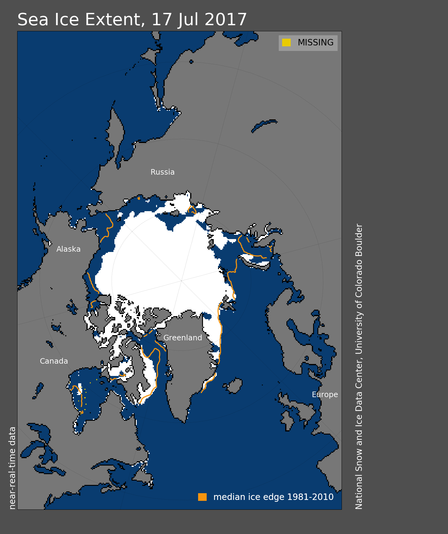
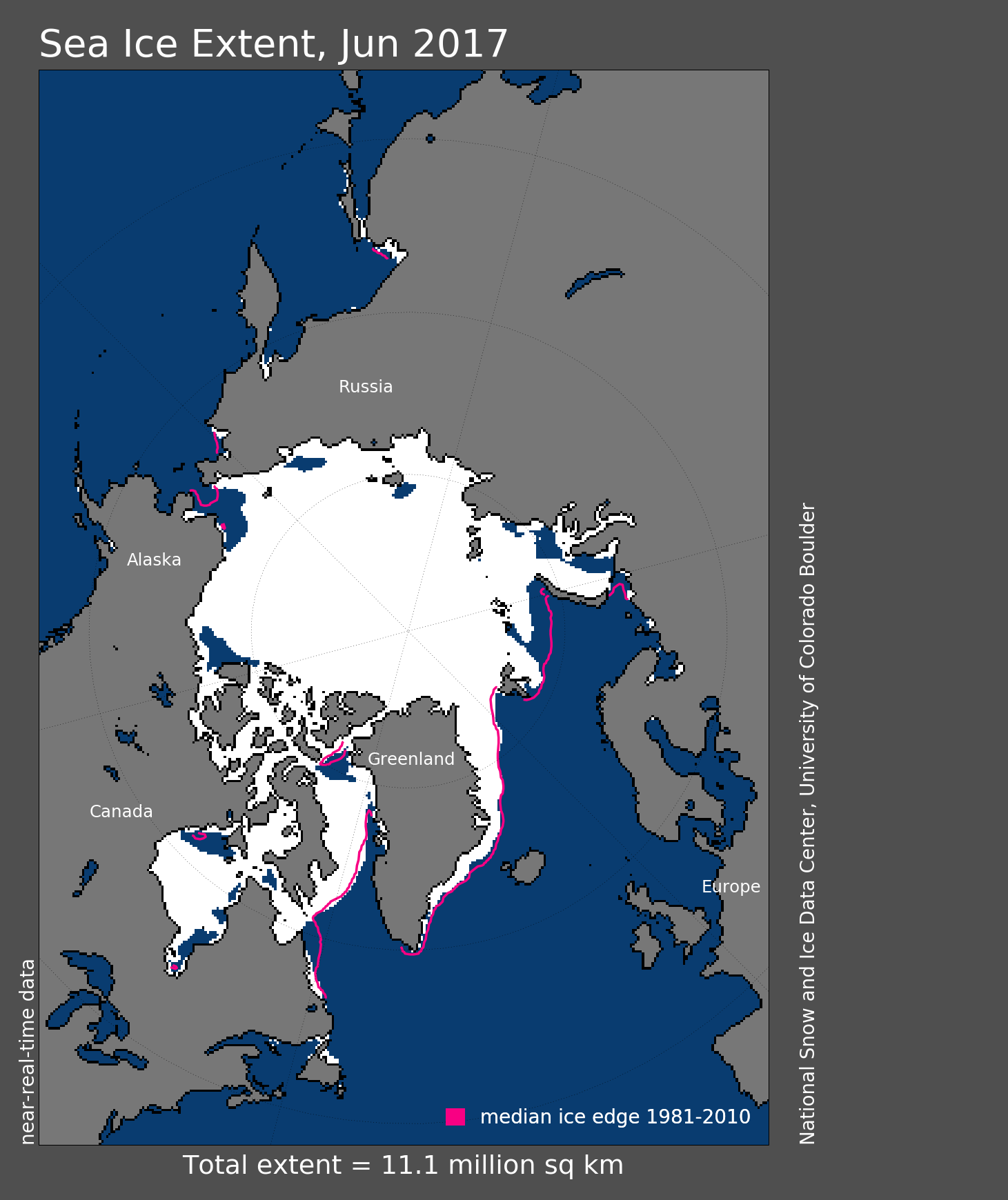
Figure 1. Arctic sea ice extent for July 17, 2017 was 7.88 million square kilometers (3.04 million square miles). The orange line shows the 1981 to 2010 average extent for that day. Sea Ice Index data. About the data

Credit: National Snow and Ice Data Center
High-resolution image

As of July 17, Arctic sea ice extent stood at 7.88 million square kilometers (3.04 million square miles). This is 1.69 million square kilometers (653,000 square miles) below the 1981 to 2010 average, and 714,000 square kilometers (276,000 million square miles) below the interdecile range. Extent was lower than average over most of the Arctic, except for the East Greenland Sea (Figure 1). Hudson Bay was nearly ice free by mid July, much earlier than is typical, but in line with what has been observed in recent years.

Conditions in context

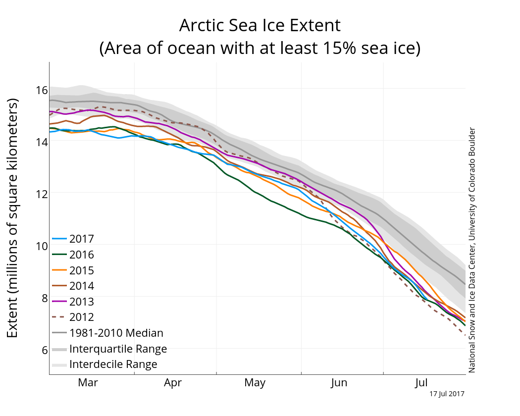
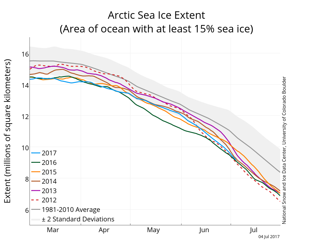
Figure 2a. The graph above shows Arctic sea ice extent as of July 17, 2017, along with daily ice extent data for five previous years. 2017 is shown in blue, 2016 in green, 2015 in orange, 2014 in brown, 2013 in purple, and 2012 as a dotted brown line. The 1981 to 2010 median is in dark gray. The gray areas around the median line show the interquartile and interdecile ranges of the data. Sea Ice Index data.

Credit: National Snow and Ice Data Center
High-resolution image

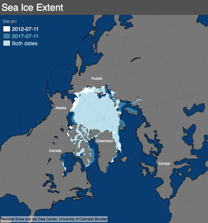
Figure 2b. This map compares sea ice extent for July 11 in 2017 and in 2012. White shows where ice occurred only in 2012, medium blue is where ice occurred only in 2017, and light blue is where ice occurred in both years.

Credit: National Snow and Ice Data Center
High-resolution image

Through the first week of July, extent closely tracked 2012 levels. The rate of decline then slowed, so that as of July 17, extent was 169,000 square kilometers (65,300 square miles) above 2012 for the same date (Figure 2a). The spatial pattern of ice extent differs from 2012, with less ice in the Chukchi and East Siberian Seas in 2017, but more in the Beaufort, Kara, and Barents Seas and in Baffin Bay (Figure 2b).

Visible imagery provides up close details

Figure 3a. This image from the NASA Moderate Resolution Imaging Spectroradiometer (MODIS) shows sea ice in the Canadian Archipelago on July 3, 2017. The blue hues indicate areas of widespread melt ponds on the surface of the ice.

Credit: Land Atmosphere Near-Real Time Capability for EOS (LANCE) System, NASA/GSFC
High-resolution image

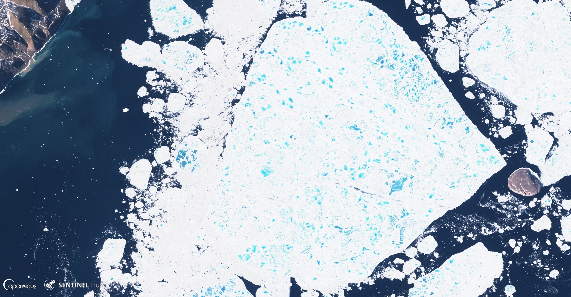
Figure 3b. The Sentinel-2 satellite captured this image of large sea ice floes in Nares Strait on July 8, 2017.

Credit: European Space Agency
High-resolution image

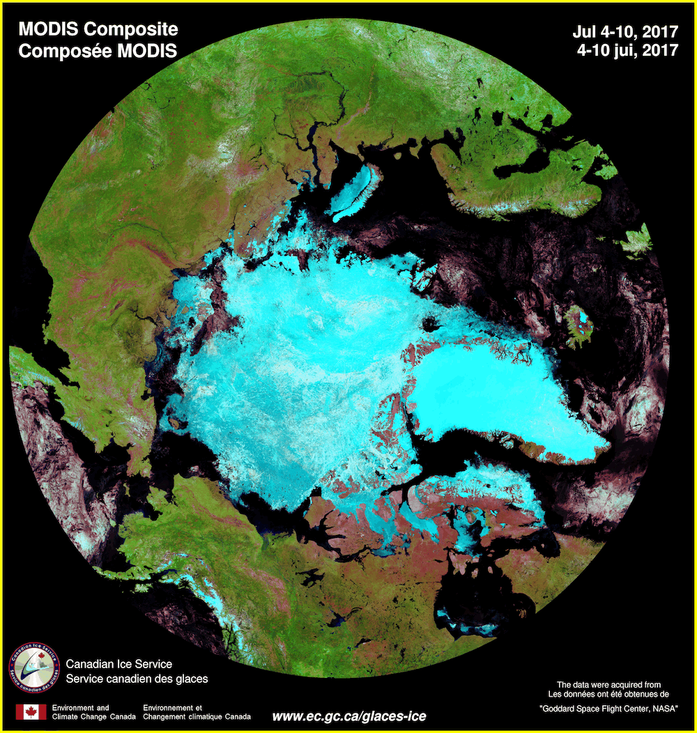
Figure 3c. This false-color composite image of the Arctic is based on NASA MODIS imagery from July 4 to 10. Most clouds are eliminated by using several images over a week, but some clouds remain, particularly over the ocean areas.

Credit: NASA/Canadian Ice Service
High-resolution image

NSIDC primarily relies on passive microwave data because it provides complete coverage—night and day, and through clouds—and because it is consistent over its long data record. However, other types of satellite data, for example visible imagery from the NASA MODIS instrument on the Aqua and Terra satellites or from the European Space Agency Sentinel 2 satellite, can sometimes provide more detail. When skies clear, details of the ice cover can be seen, including leads, individual ice floes and melt ponds. For example, on July 3 in the Canadian Archipelago, 1-kilometer resolution MODIS imagery shows that the ice surface has a distinctive blueish hue due to the presence of melt ponds on the surface (Figure 3a). Higher resolution Sentinel-2 imagery (10 meters, Figure 3b) on the other hand provides up close detail on individual melt ponds on the ice floes.

The Arctic is a cloudy place, and generally, it is difficult to obtain a clear-sky image of the entire region. However, if images are compiled, or composited, over several days, most of the region may have at least some clear sky. This approach can yield a composite image that is mostly cloud-free. The Canadian Ice Service uses this approach to create a weekly nearly cloud-free composite image of the Arctic (Figure 3c). However, because the ice cover moves (typically several kilometers per day) and melts (during the summer), over the week-long composite period, fine details that can be seen in the daily imagery are not as evident because they have been “smeared” out over the week.

An ice-diminished Arctic

In response to diminishing ice extent, the US Navy has been holding a semi-annual symposium to bring together scientists, policy makers, and others to discuss the sea ice changes and their impacts. The seventh Symposium is taking place this week in Washington, DC, and will be attended by NSIDC scientists Mark Serreze, Walt Meier, Florence Fetterer, and Ted Scambos.

Tendency for warmer winters is increasing

A new study published this week in Geophysical Research Letters by Robert Graham at the Norwegian Polar Institute shows that warm winters in the Arctic are becoming more frequent and lasting for longer periods of time than they used to. Warm events were defined by when the air temperatures rose above -10 degrees Celsius (14 degrees  Fahrenheit). While this is still well below the freezing point, it is 20 degrees Celsius (36 degrees Fahrenheit) higher than average. The last two winters have seen temperatures near the North Pole rising to 0 degrees Celsius. While an earlier study showed that winter 2015/2016 was the warmest recorded at that time, the winter of 2016/2017 was even warmer.

Reference

Graham, R. M., L. Cohen, A. A. Petty, L. N. Boisvert, A. Rinke, S. R. Hudson, M. Nicolaus, and M. A. Granskog. 2017. Increasing frequency and duration of Arctic winter warming events, Geophys. Res. Lett., 44, doi:10.1002/2017GL073395.

Contrasting with the fairly slow start to the melt season in May, June saw the ice retreat at a faster than average rate. On July 2, Arctic sea ice extent was at the same level recorded in 2012 and 2016. In 2012, September sea ice extent reached the lowest in the satellite record. As a new feature to Arctic Sea Ice News and Analysis, NSIDC now provides a daily updated map of ice concentration in addition to the daily map of ice extent.

Overview of conditions

Figure 1. Arctic sea ice extent for June 2017 averaged 11.06 million square kilometers (4.27 million square miles). The magenta line shows the 1981 to 2010 average extent for that month. Sea Ice Index data. About the data

Credit: National Snow and Ice Data Center
High-resolution image

Arctic sea ice extent for June 2017 averaged 11.06 million square kilometers (4.27 million square miles), the sixth lowest in the 1979 to 2017 satellite record. The average June 2017 extent was 900,000 square kilometers (348,000 square miles) below the 1981 to 2010 long-term average, and 460,000 square kilometers (178,000 square miles) above the previous record low set in 2016.

Continuing the pattern seen in May, sea ice extent at the end of the month remained below average in the Chukchi Sea and in the Barents Sea. Ice extent was at average levels in the Greenland Sea. Areas of low concentration ice have developed along the ice edge and coastal seas.

Based on imagery from the Moderate Resolution Imaging Spectroradiometer (MODIS) aboard the NASA Terra and Aqua satellites, summer melt ponds atop the ice cover were somewhat slow to develop. However, there is now widespread melt pond coverage in the Canadian Archipelago and the Laptev and East Siberian Seas. Data from the Advanced Microwave Scanning Radiometer 2 (AMSR-2) instrument analyzed by the University of Bremen, as well as MODIS imagery, indicate that melt ponds have also developed over the Central Arctic Ocean. Researchers in Dease Strait in Northern Canada have observed melt ponds forming about two weeks earlier than average. Melt ponds are important as they decrease the albedo or reflectivity of the ice surface, which hastens further melt.

Conditions in context

Figure 2. The graph above shows Arctic sea ice extent as of July 4, 2017, along with daily ice extent data for five previous years. 2017 is shown in blue, 2016 in green, 2015 in orange, 2014 in brown, 2013 in purple, and 2012 in dashed red. The 1981 to 2010 median is in dark gray. The gray areas around the median line show the interquartile and interdecile ranges of the data. Sea Ice Index data.

Credit: National Snow and Ice Data Center
High-resolution image

The rate of decline in ice extent was fairly steady through the month, and the average rate of decline of 81,800 square kilometers (31,600 square miles) per day was slightly faster than the 1981 to 2010 long-term average of 56,300 square kilometers (21,700 square miles) per day. On July 2, extent was the same as that recorded in 2012 and 2016. The year 2012 ended up with the lowest September extent in the satellite record.

June air temperatures were modestly above average (1 to 3 degrees Celsius or 2 to 5 degrees Fahrenheit) in a band spanning the Arctic Ocean roughly centered along the date line and the prime meridian. This contrasts with below-average temperatures over the eastern Beaufort Sea and Canadian Arctic Archipelago and the Barents and Laptev Seas (1 to 3 degrees Celsius, 2 to 5 degrees Fahrenheit). Atmospheric pressures at sea level were below-average over the Kara Sea and extending north of the Laptev Sea.

June 2017 compared to previous years

Figure 3. Monthly June ice extent for 1979 to 2017 shows a decline of 3.7 percent per decade.

Credit: National Snow and Ice Data Center
High-resolution image

The linear rate of decline for June is 44,300 square kilometers (17,100 square miles) per year, or 3.7 percent per decade.

Ice thickness

Figure 4. This figure shows that sea ice thicknesses for May 2017 were below the 2000 to 2015 average over most of the Arctic Ocean (areas in blue) except for the region north and west of the Svalbard archipelago (areas in red).

Credit: University of Washington Pan-Arctic Ice Ocean Modeling and Assimilation System
High-resolution image

The University of Washington Seattle Pan-Arctic Ice Ocean Modeling and Assimilation System (PIOMAS) regularly produces maps of ice thickness anomalies (departures from the long-term average). PIOMAS is based on a coupled ice-ocean model that is driven by data from an atmospheric reanalysis, and also assimilates data on observed ocean conditions and ice thickness (e.g., from NASA IceBridge). The PIOMAS analysis suggests that, relative to the average over the period 2000 to 2015, ice thickness for May 2017 (when the melt season was just beginning) was below average over most of the Arctic Ocean, especially in the Chukchi Sea and north of the Canadian Arctic Archipelago. A small region with above-average ice thickness is depicted over the Atlantic side of the Arctic north and west of the Svalbard Archipelago, and in the Greenland Sea. Starting the melt season with below-average ice thickness raises the likelihood of having especially low September ice extent.

Freezing degree days and ice thickness

Figure 5. The figure shows departures from average in cumulate freezing degree days, extending from July 1 for a given year through July 1 of the next year, along with the range, 15th through 85th percentile and 30th to 70th percentile values over the base period 1981 through 2010.

Credit: National Snow and Ice Data Center
High-resolution image

Cumulative Freezing Degree Days (FDD) is a simple measure of how cold it has been and for how long. Cumulative FDD is the sum of daily mean temperatures below zero from some start date. Here we start on July 1. Cumulative FDD is related to ice thickness because, on average, years with longer periods of temperatures below freezing will have more ice growth. A simple empirical model that has been used by scientists relates ice thickness to the square root of cumulative FDD.

Anomalies (departures from the average) in cumulative FDD illustrate the coldness of a given period relative to the long-term average (1981 to 2010). Figure 5 shows that most of the period from July 2016 to July 2017 was extremely mild and was milder (less cold) than both 2006 to 2007 and 2011 to 2012. September of both 2007 and 2012 ended up with very low September sea ice extent. This is consistent with below-average ice thickness seen in the PIOMAS data. Although conditions cooled in May and June, this likely had little impact on ice thickness. This is because ice in the Arctic reaches its maximum thickness earlier in the season during March or April. As noted earlier, ice retreated at a fast rate throughout June. This is likely linked to a thinner than average ice cover as seen in the PIOMAS analysis.

Sudden Antarctic sea ice decline in late 2016

A slight decrease in the rate of sea ice growth at the end of June brought Antarctic sea ice extent back to daily record lows. Sea ice extent in the Bellingshausen, eastern Amundsen, and western Ross Seas was below average.

Our post on December 2016 ice conditions highlighted a precipitous drop in Antarctic sea ice extent in the Weddell and Ross Sea sectors during September, October, and November of 2016. A recent study by John Turner and colleagues links this pattern of sea ice decline to a series of strong storms, marked by long periods of warm winds from the north. These changing weather conditions are associated with large shifts in the Southern Annual Mode index (SAM index).

Further reading

Turner, J., T. Phillips, G. J. Marshall, J. S. Hosking, J. O. Pope, T. J. Bracegirdle, and P. Deb. 2017. Unprecedented springtime retreat of Antarctic sea ice in 2016, Geophysical Research Letters, 44, doi:10.1002/2017GL073656.