Arctic sea ice extent continues its seasonal decline. Through most of June the pace of decline was near average, but increased towards the end of the month.

Overview of conditions

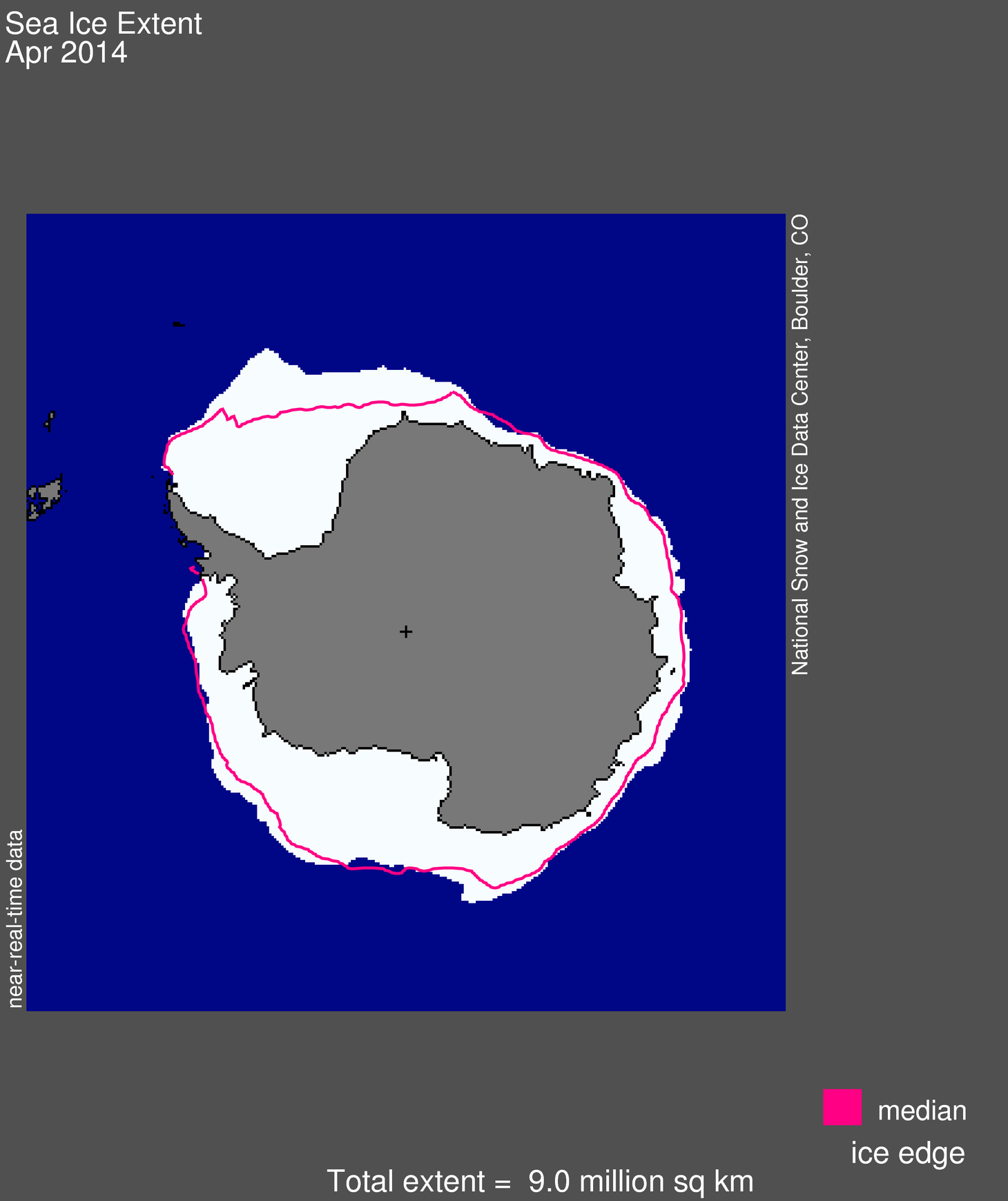
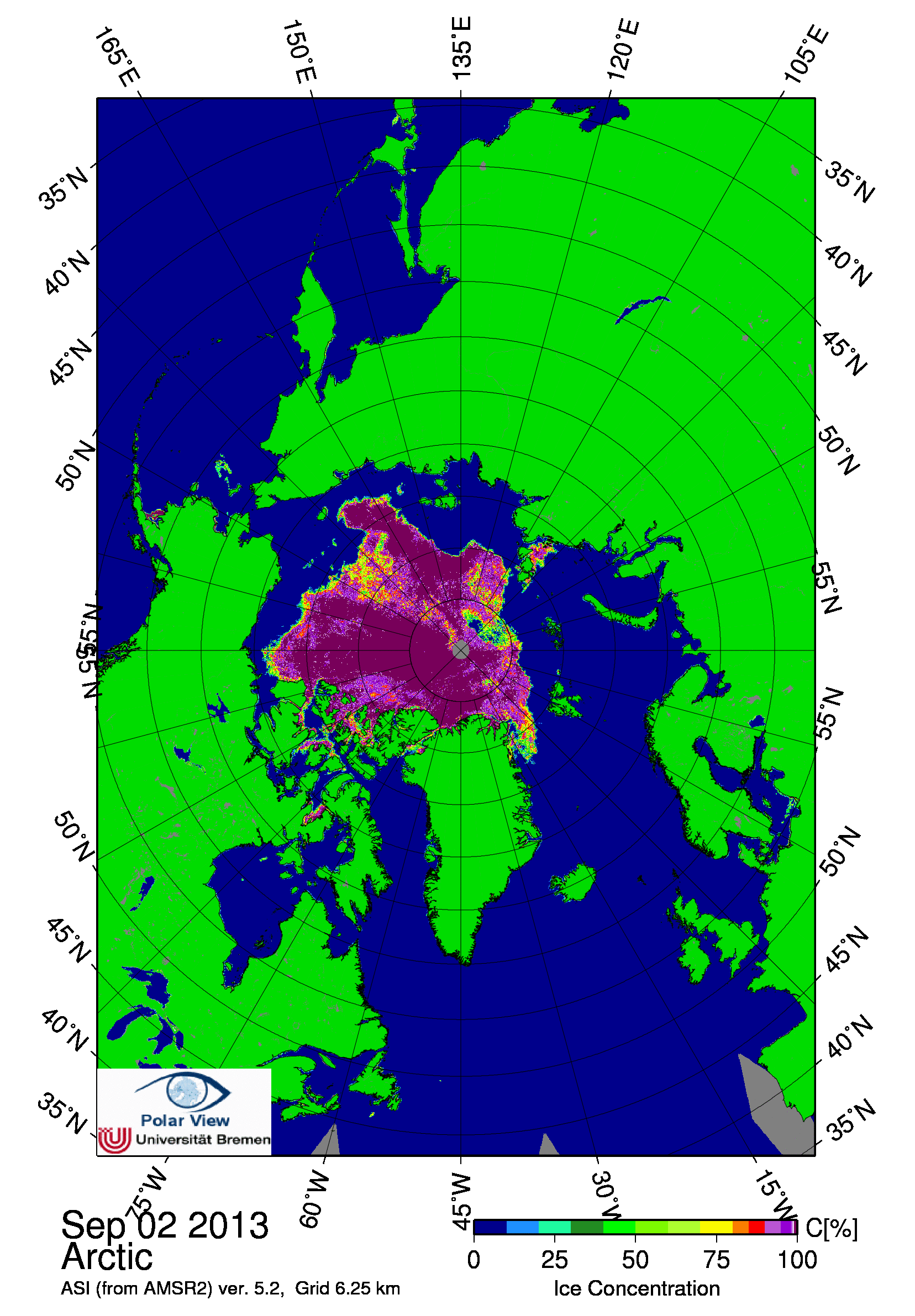
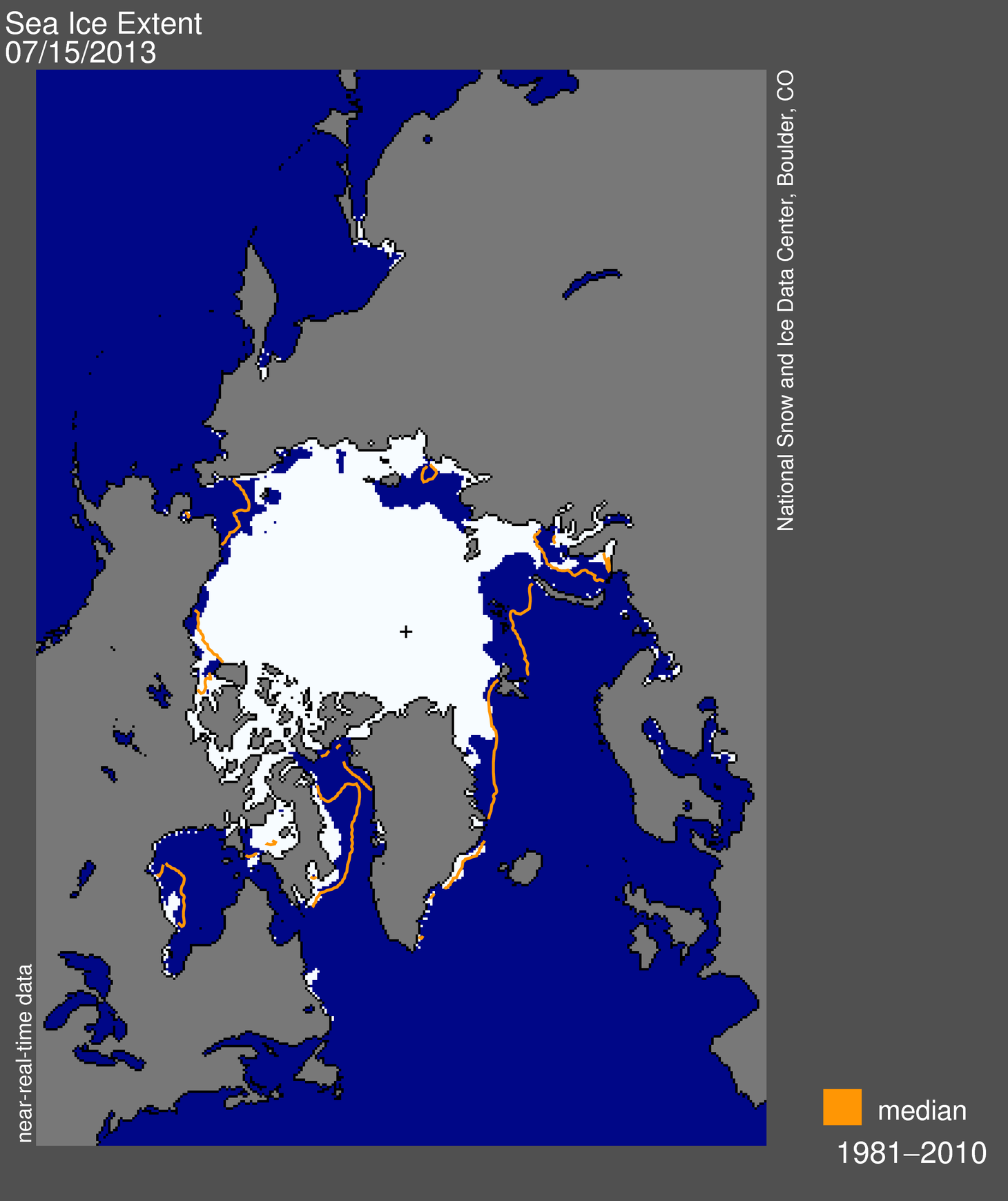
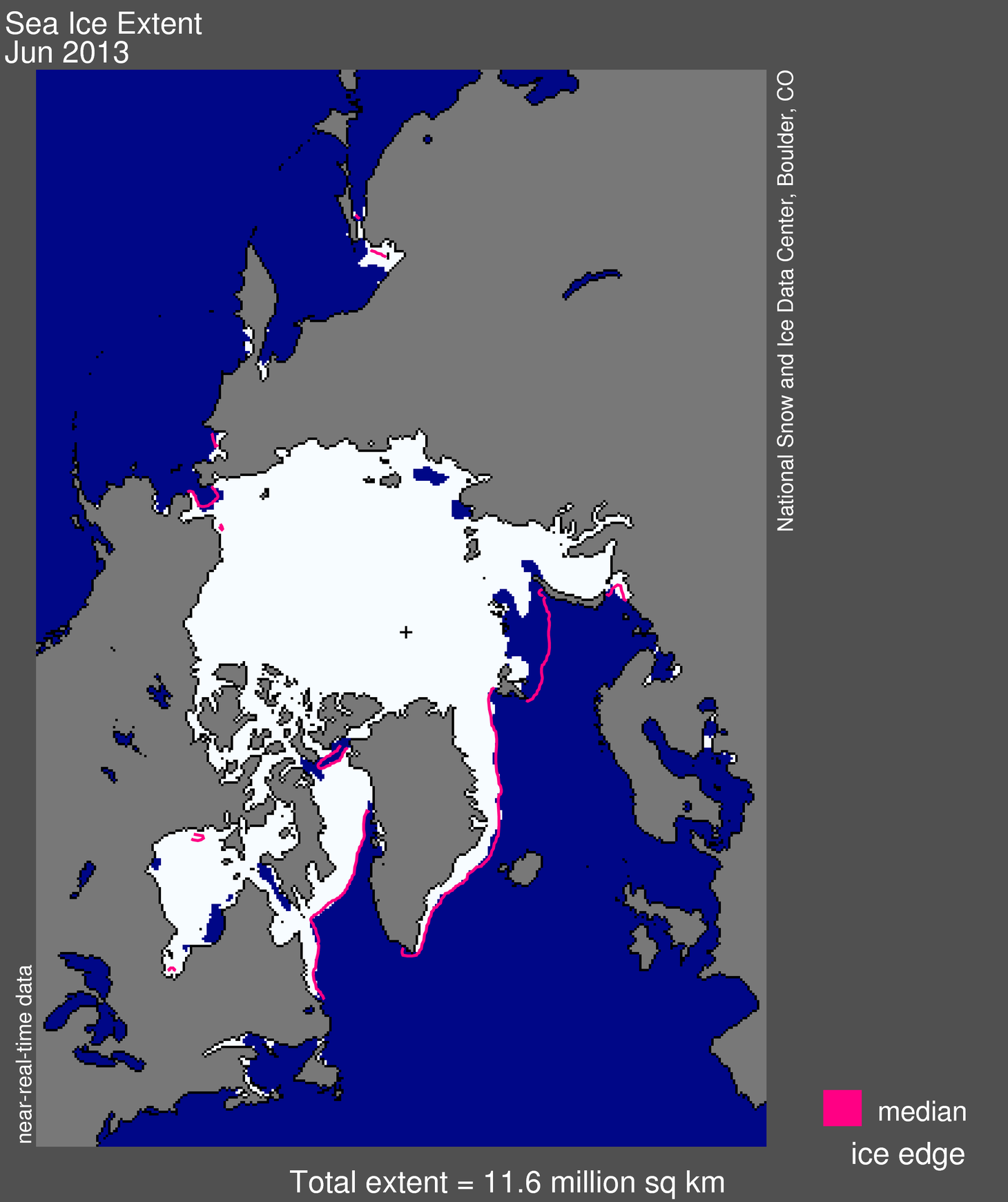
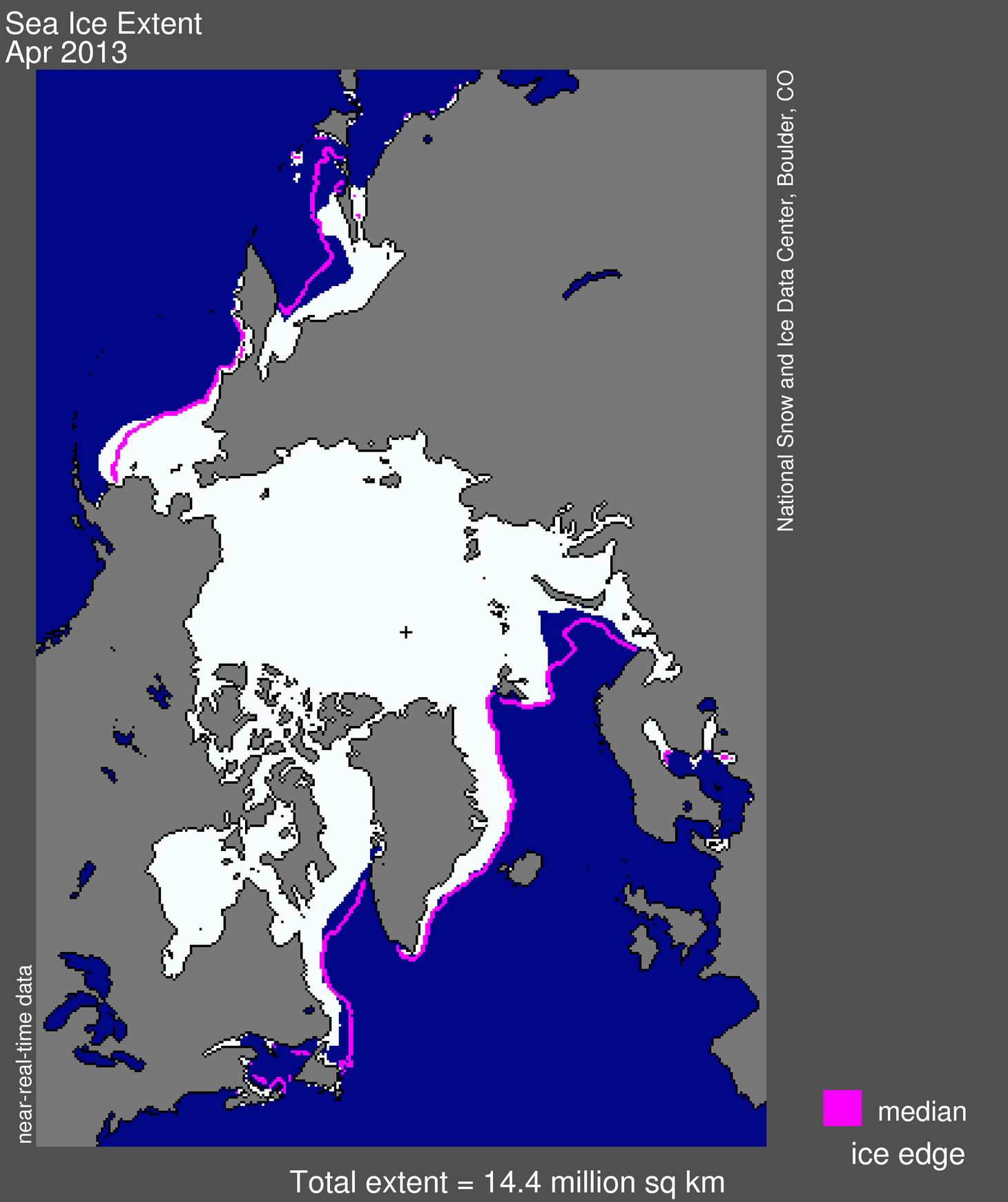
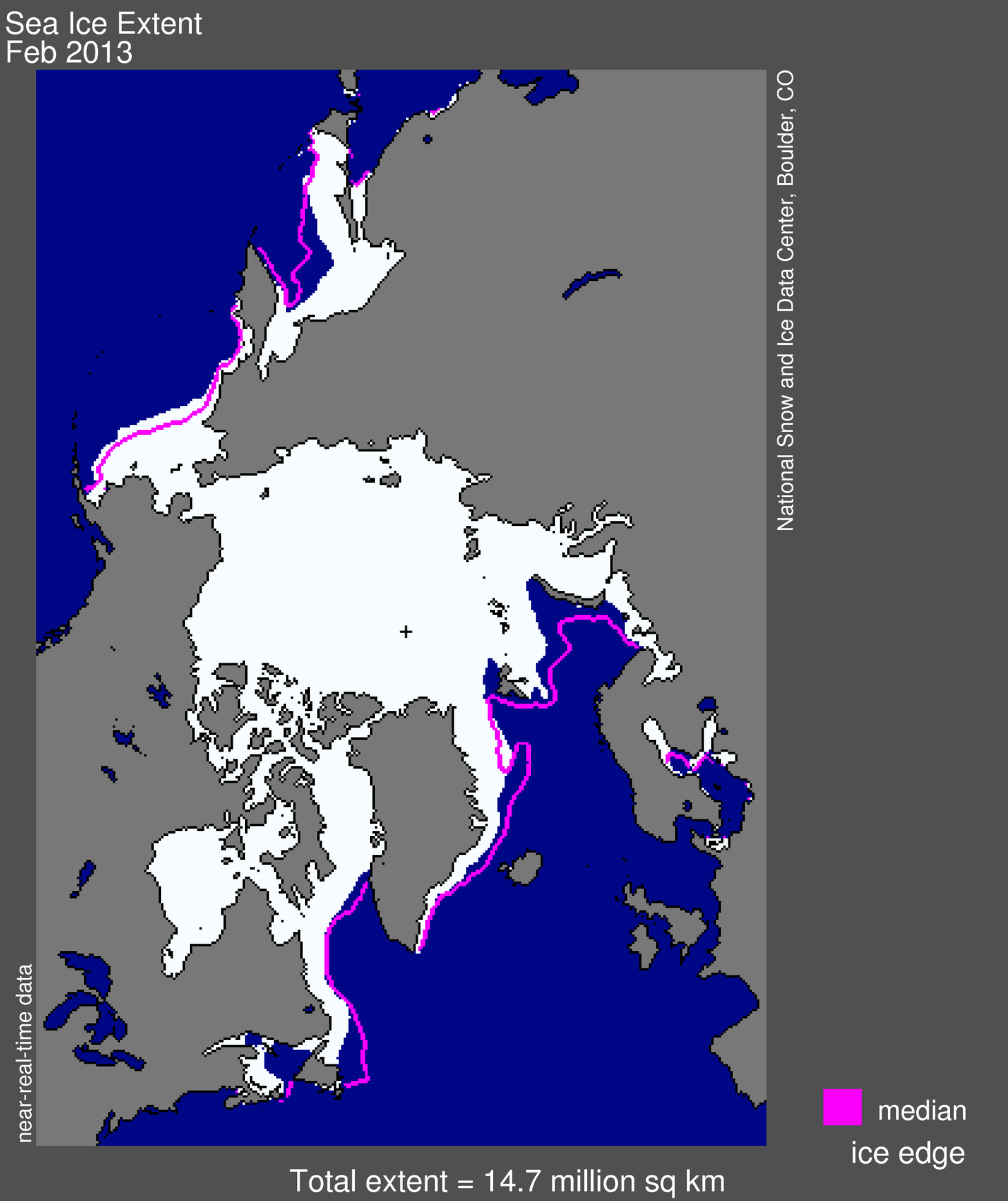
Figure 1. Arctic sea ice extent for June 2014 was 11.31 million square kilometers (4.37 million square miles). The magenta line shows the 1981 to 2010 median extent for that month. The black cross indicates the geographic North Pole. Sea Ice Index data. About the data

Credit: National Snow and Ice Data Center
High-resolution image

June 2014 averaged 11.31 million square kilometers (4.37 million square miles). This is 580,000 square kilometers (224,000 square miles) below the 1981 to 2010 average for the month.

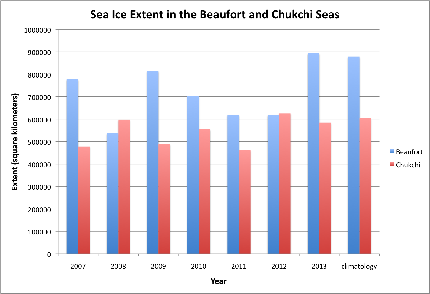
Large areas of open water quickly opened up in the Laptev Sea at the beginning of June and continued to expand through the month. The southern part of the Beaufort Sea has also opened and melt ponds are apparent on the open drift first-year ice and extending into the pack ice (see Figure 5 below). Nevertheless, ice extent in this region continued to be above the levels of recent years through much of the month. Extent was lower than average in the Barents Sea, Hudson Bay, and the East Greenland Sea, but higher than in recent years in the Kara Sea.

Conditions in context

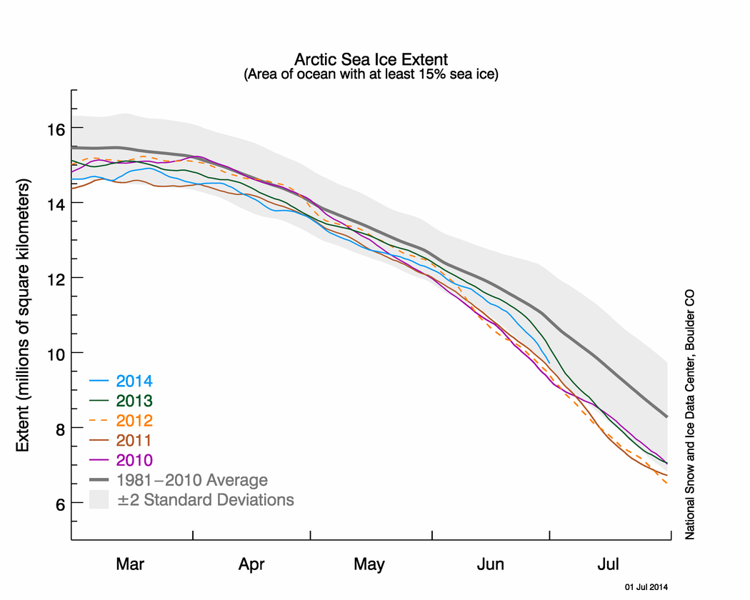
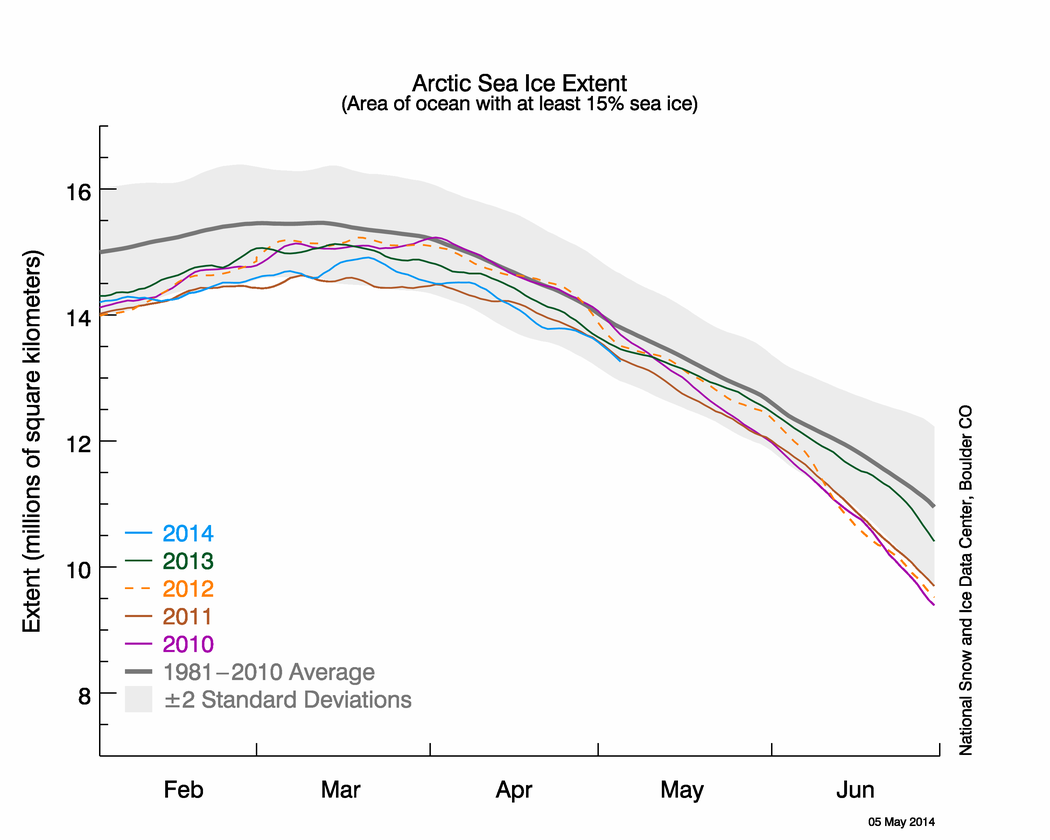
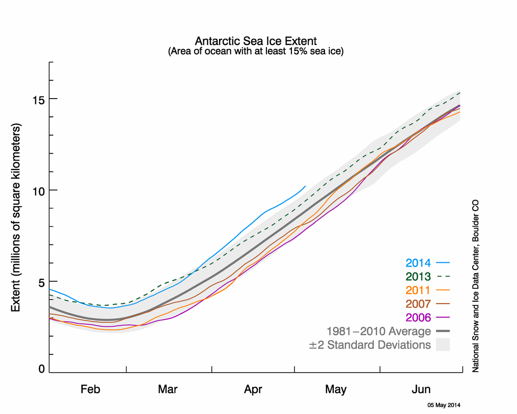
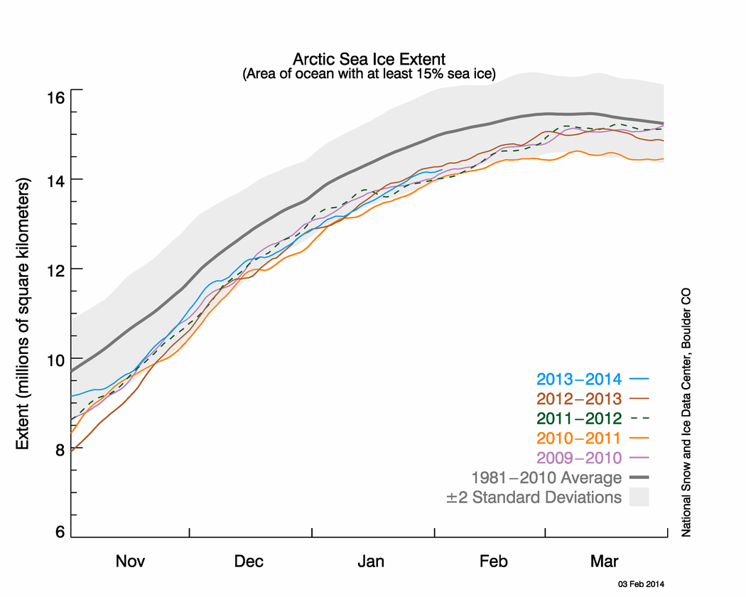
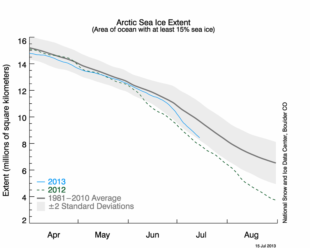
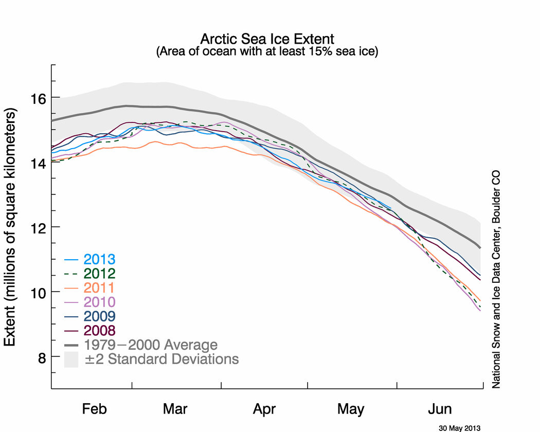
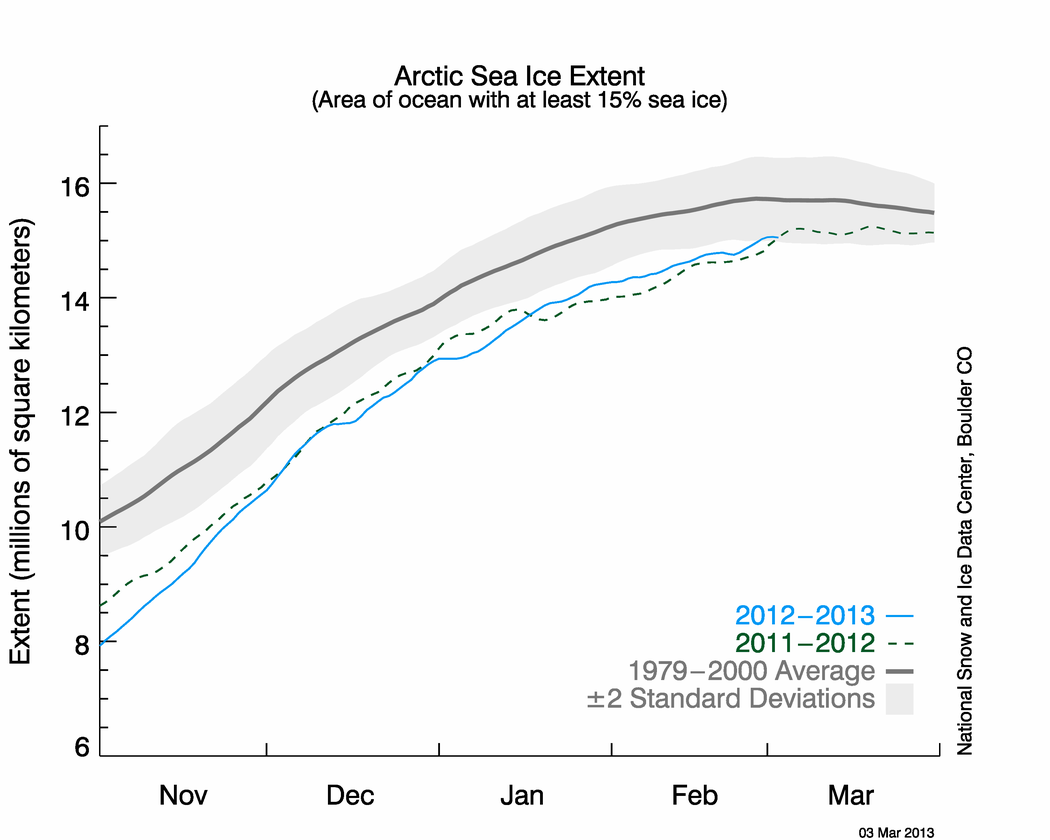
Figure 2. The graph above shows Arctic sea ice extent as of July 1, 2014, along with daily ice extent data for four previous years. 2014 is shown in blue, 2013 in green, 2012 in orange, 2011 in brown, and 2010 in purple. The 1981 to 2010 average is in dark gray. Sea Ice Index data.

Credit: National Snow and Ice Data Center
High-resolution image

Ice extent during June declined by an average of 78,900 square kilometers (30,500 square miles) per day, faster than the 1981 to 2010 average June rate of 57,200 square kilometers (22,100 square miles) per day. Last March’s relatively low maximum extent helped set the stage for June’s low extent. June is a month that has seen large variability in the rate of ice loss in recent years. In 2012, a period of rapid acceleration occurred during the first half of the month, kick-starting the decline towards the eventual record low extent that September. So far, 2014 has failed to match the 2012 loss rates. However, ice extent on June 30th came within 300,000 square kilometers (115,800 square miles) of that in 2012. The 2014 rate of ice decline also accelerated toward the end of June as wide areas of low-concentration ice on the peripherial areas of the Arctic Ocean opened up, especially in the Hudson and Baffin bays. This increased rate of loss is typical of late June and early July, and is visible in the 30-year mean trend for Arctic sea ice (see the ChArctic interactive sea ice chart).

June 2014 compared to previous years

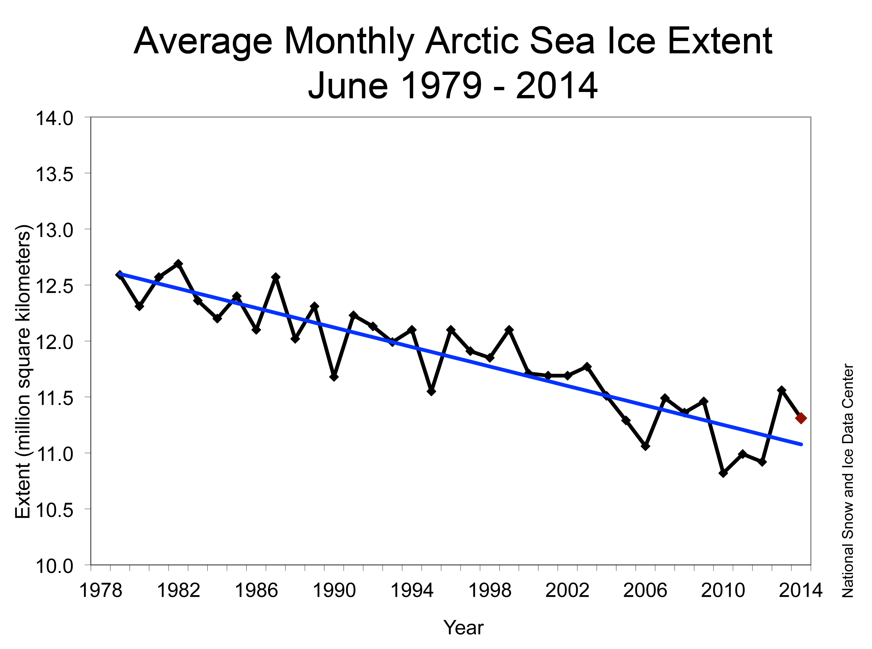
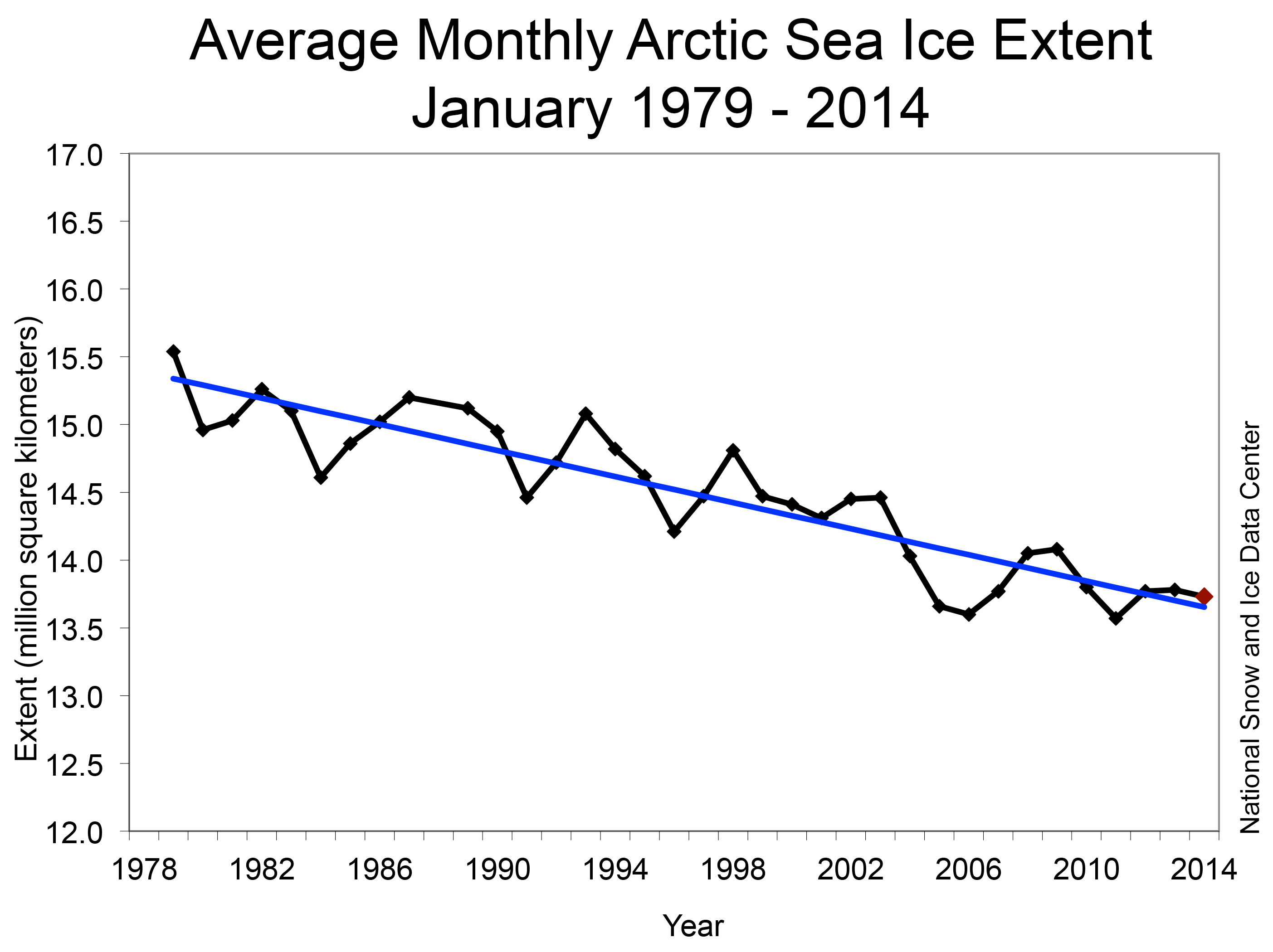
Figure 3. Monthly June ice extent for 1979 to 2014 shows a decline of 3.6% per decade relative to the 1981 to 2010 average.

Credit: National Snow and Ice Data Center
High-resolution image

June 2014 is the 6th lowest Arctic sea ice extent in the satellite record, 490,000 square kilometers (189,000 square miles) above the previous record low in June 2010. The monthly linear rate of decline for June is 3.6% per decade.

A cooler June

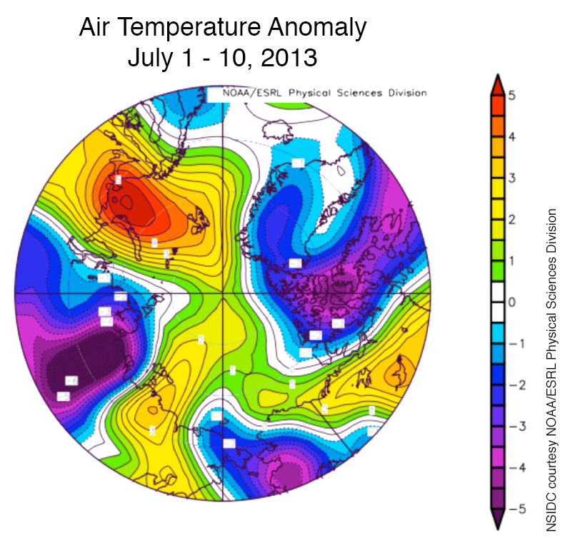
Figure 4. These images show air temperature anomalies for June 2012, 2013, and 2014 at the 925 Mb level (approximately 3,000 feet above sea level).

Credit: NOAA/ESRL Physical Sciences Division
High-resolution image

At the 925 mb level (approximately 3000 feet above sea level) average June temperatures over parts of the Arctic Ocean were from 1 to 2 degrees Celsius (2 to 4 degrees  Fahrenheit) below the 1981 to 2010 average, but with a warming trend over the latter half of the month; the last week of June saw temperatures of 2 to 4 degrees Celsius (4 to 7 degrees Fahrenheit) above average over the central Arctic Ocean. June 2013 was also slightly cooler than average.This is in stark contrast to the unusually warm summers of many recent years, particularly 2012 and 2007 when air temperatures over the Arctic Ocean were up to 4 to 6 degrees Celsius (7 to 11 degrees Fahrenheit), respectively, above average.

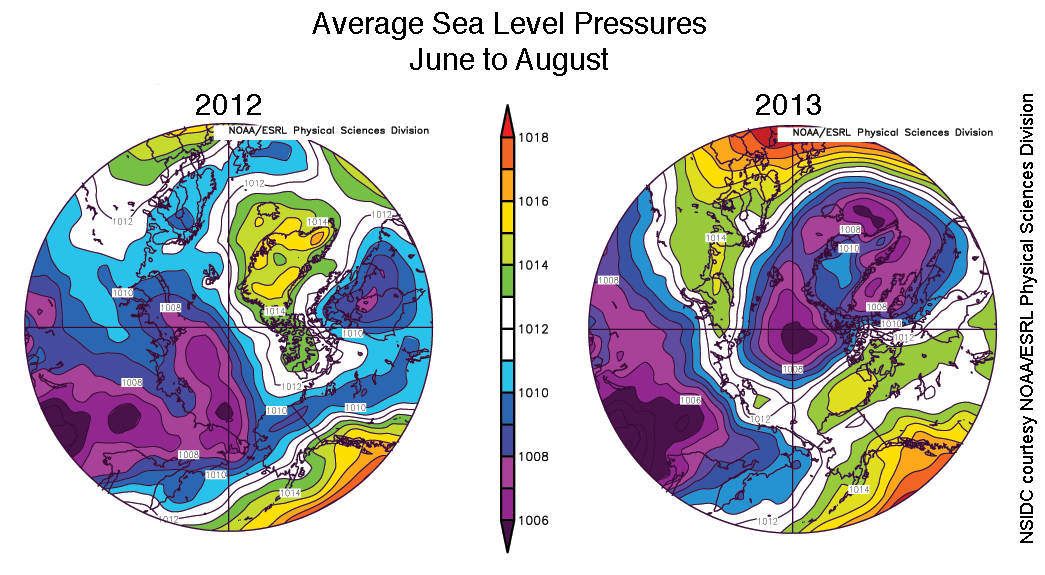
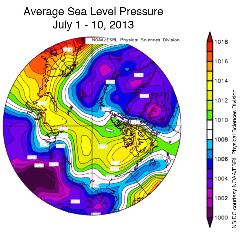
The cool conditions in June 2013 were attributed to a generally cyclonic pattern of atmospheric circulation. However, by late June 2014 the more typical pattern of high pressure over the Beaufort Sea had developed, coupled with low pressure over Alaska and Eurasia.

Landsat 8 expands Arctic Sea Ice coverage

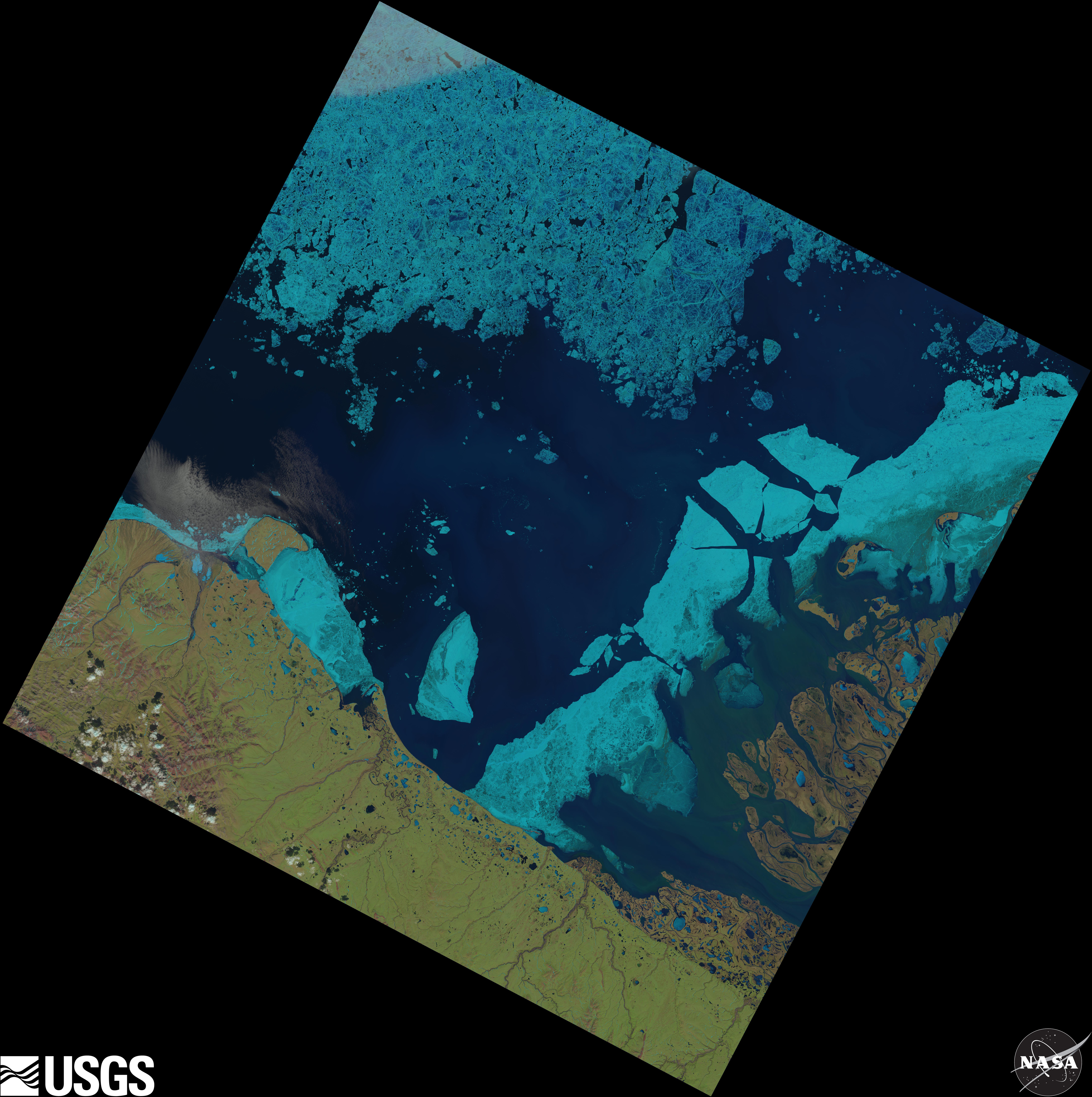
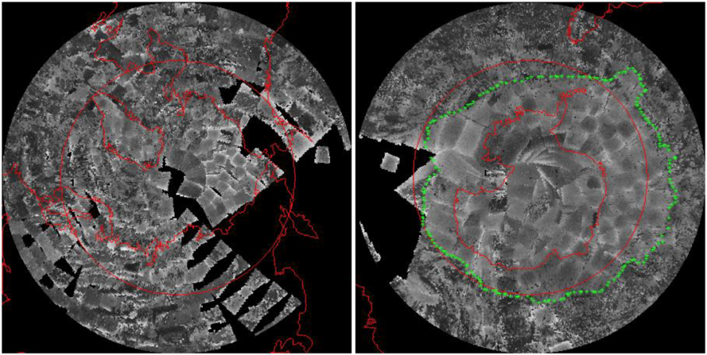
Figure 5. This Landsat 8 image of the Beaufort Sea and MacKenzie River Delta was acquired on June 16 , 2014. The approximately true-color image shows abundant surface melt and melt ponds, fast ice break up, and coastal features of the springtime Arctic. The image is 185 kilometers (115 miles) on each side.

Credit: National Snow and Ice Data Center/USGS/NASA/Landsat 8.
High-resolution image

Landsat 8, launched in February of 2013, has been regularly acquiring images of the world’s daylit land surface since May of that year. The mission recently increased the pace of image acquisition, covering nearly all available daylit areas each day, and expanded coverage of sea ice areas in the Arctic and coastal areas of Greenland (the latter with ascending node, or evening hour, coverage). Coverage for the Arctic Ocean is focused on the far western and far eastern Arctic, that is, the Beaufort, Chukchi, and East Siberian Sea, although substantial coverage of sea ice is included in the acquisition of all Arctic land areas. Ascending (evening) and decending (morning, the typical acquisition time) coverage of coastal Greenland permits better tracking of glacier flow and in particular sea ice break-up and glacier retreat in the fjord areas.

The images, and the historical (somewhat variable) record of Arctic coverage provide information on ice type, surface melting and melt ponds, ice motion, coastal fast ice break-up, lead fraction and shear zones within the ice.

More on seasonal thickness evolution of Arctic sea ice

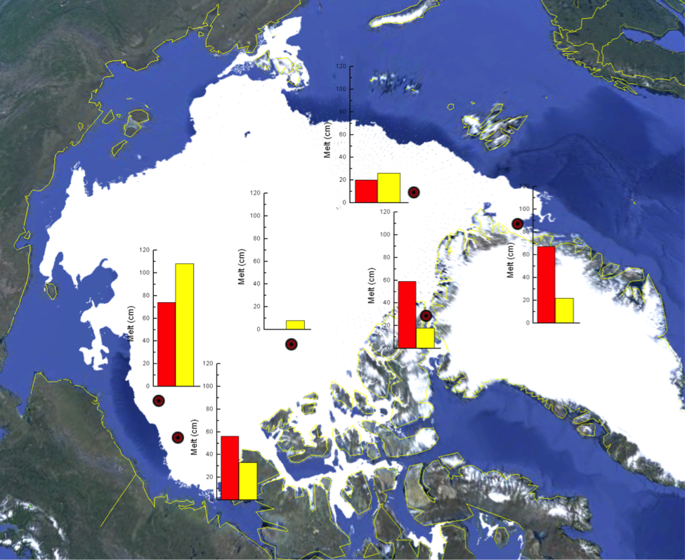
Figure 6. Air temperature (top), ice temperature and thickness (middle), and water temperature (bottom) from the U.S. Navy’s Office of Naval Research (ONR) Marginal Ice Zone project ice mass balance buoys for March to June 2014.

Credit: U.S. Navy’s Office of Naval Research (ONR) Marginal Ice Zone project
High-resolution image

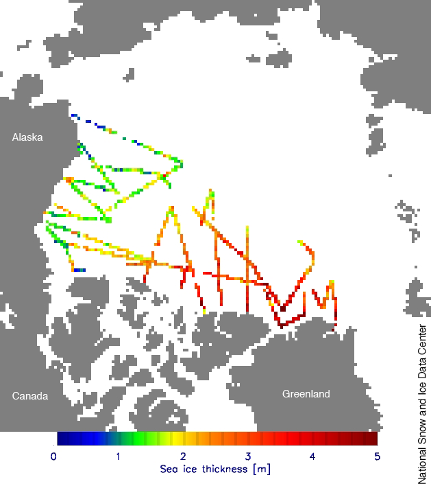
As noted in last month’s post, satellite and airborne sensors are now able to provide good coverage of the Arctic ice thickness. However, as with any remote sensing estimate, the observations come with uncertainty. Direct measurements, even though they do not provide wide-coverage, are important for validation. They can also provide a useful indication of general ice conditions (thickness, temperature) at the beginning of the ice season. Such direct observations, in concert with available satellite and airborne data, can improve seasonal forecasts of sea ice, such as those provided in the recently released Sea Ice Outlook.

In March, the U.S. Navy’s Office of Naval Research (ONR) Marginal Ice Zone project deployed three clusters of mass balance buoys on the sea ice, complementing ongoing similar deployments by the U.S. Army Cold Regions Research and Engineering Laboratory. These mass balance buoys not only provide a simple thickness measurement, but can also provide a time series of the evolution of the ice, both at the top and bottom surface. The ONR buoys additionally include air temperatures sensors, which are useful for monitoring atmospheric conditions, as well as temperatures through and below the ice.

ONR deployed three clusters of buoys in the Beaufort Sea at three different latitudes.  Initial ice thickness at the sites was between 1.5 and 2 meters (5 and 6.5 feet). During April and May, there were brief incursions of above freezing air temperatures leading to some melt, but temperatures mostly remained below freezing until early June. All three clusters show continuous above freezing air temperatures starting by the second week of June. With the higher temperatures, melt has commenced on both the top and bottom surfaces.

The Beaufort Sea has been a region of dramatic summer ice loss in recent years, particularly 2012, with regions dominated by thicker, multi-year ice melting out completely. While vigorous melt has begun, it remains to be seen how the ice cover will evolve over the rest of the melt season.

Since reaching its annual maximum extent on March 21, Arctic sea ice extent has declined somewhat unevenly, but has consistently been well below its average 1981 to 2010 extent. While the rate of Arctic-wide retreat was rapid through the first half of April, it has subsequently slowed down. However, ice breakup was quite early in the Bering Sea, presenting difficulties for gold dredging operations and seal hunters in the region. In the Antarctic, sea ice continued to reach record high extents.

Overview of conditions

Figure 1. Arctic sea ice extent for April 2014 was 14.14 million square kilometers (5.46 million square miles). The magenta line shows the 1981 to 2010 median extent for that month. The black cross indicates the geographic North Pole. Sea Ice Index data. About the data

Credit: National Snow and Ice Data Center
High-resolution image

Arctic sea ice extent for April 2014 averaged 14.14 million square kilometers (5.46 million square miles). This is 610,000 square kilometers (236,000 square miles) below the 1981 to 2010 average extent, and 270,000 square kilometers (104,000 square miles) above the record April monthly low, which occurred in 2007. While the rate of ice loss was rapid through the first half of April, it subsequently slowed down. The rate of ice loss averaged for the month was 30,300 square kilometers per day (11,700 square miles per day), which is slower than the average rate of 38,400 square kilometers per day (14,800 square miles per day) over the period 1981 to 2010. As of May 4, 2014, extent was below average in the Barents Sea, Sea of Okhotsk, and the Bering Sea, and slightly above average in Baffin Bay.

Conditions in context

Figure 2. The graph above shows Arctic sea ice extent as of May 5, 2014, along with daily ice extent data for four previous years. 2014 is shown in blue, 2013 in green, 2012 in orange, 2011 in brown, and 2010 in purple. The 1981 to 2010 average is in dark gray. Sea Ice Index data.

Credit: National Snow and Ice Data Center
High-resolution image

Air temperatures at the 925 hPa level (roughly 3,000 feet above the surface) were from 1 to 3 degrees Celsius (2 to 5 degrees Fahrenheit) above the 1981 to 2010 average over most of the Arctic Ocean, most notably over the East Siberian Sea and in the Bering Strait region. This contrasts with the region centered over Svalbard, where temperatures were up to about 2 degrees Celsius (4 degrees Fahrenheit) below average. The atmospheric circulation pattern as averaged over the month was somewhat unusual, featuring a large area of low sea level pressure centered over the Laptev and Barents seas. Pressures in this region were up to 16 hPa below the 1981 to 2010 average. The transport of warm air from the south along the eastern side of the low pressure area is consistent with the above average temperatures over the East Siberian Sea. The Arctic Oscillation (AO) was in its positive phase through the first three weeks of April, and then regressed to a modestly negative phase.

April 2014 compared to previous years

Figure 3. Monthly April ice extent for 1979 to 2014 shows a decline of 2.4% per decade relative to the 1981 to 2010 average.

Credit: National Snow and Ice Data Center
High-resolution image

Average ice extent for April 2014 was the fifth lowest for the month in the satellite record. Through 2014, the linear rate of decline for April ice extent is -2.4% per decade relative to the 1981 to 2010 average.

Early breakup in the Bering Sea

Figure 4. This image of the Bering Strait, taken by the NASA Moderate Resolution Imaging Spectroradiometer (MODIS) on April 29, shows the sea ice pack breaking up in the Bering Strait.

Credit: Sea Ice for Walrus Outlook/Land Atmosphere Near-Real Time Capability for EOS (LANCE) System, NASA/GSFC

High-resolution image

The anomalously low sea ice conditions in the Bering Sea are partially a result of low winter ice cover (see our March 3, 2014 post) and an unusually early breakup of sea ice. The Fairbanks Daily News Miner reported that the unusually early breakup of ice in the Bering Sea forced several gold dredging operations to act quickly to get their equipment off the coastal sea ice, which is used as a platform to work shallow seabed gold deposits. Seal hunters were also impacted by the early breakup, in some cases abandoning their snowmobiles on the ice as it became unstable or impassable. The snowmobiles were later recovered by boat. The SEARCH Sea Ice for Walrus Outlook provides weekly updates on sea ice conditions within the Bering Sea region for hunters, local communities and others interested in local ice conditions.

Importance of spring melt ponds

Figure 5. This graph compares actual September sea ice extent to predictions of sea ice extent based on melt pond fraction, integrated over the period 1 May – 25 June. Predicted ice extent is verified by use of SSM/I data for the period 1979–2013. Prediction error is 0.36 million square kilometers for hindcasts and 0.44 million square kilometers for forecasts.

Credit: D. Schröder et al., Nature Climate Change
High-resolution image

In spring, snow covers the sea ice on the Arctic Ocean and the albedo, or surface reflectivity, is high. As air temperatures increase, this snow begins to melt and collect on top of the sea ice. Dark melt ponds form, absorbing more energy from the sun than the adjacent bright snow and ice surfaces. A paper recently published in Nature Climate Change by Schröder et al. suggests that the fraction of melt ponds during May plays an important role in how much ice will be left at the end of the melt season in September. Melt ponds enhance the absorption of the sun’s energy by the sea ice pack, melting more snow and ice and further increasing the melt pond fraction. If melt ponds are widespread across the Arctic Ocean by mid-June and into July, under the 24-hour Arctic summer sunlight, then their effect is increased.

The size and number of melt ponds on sea ice are in part governed by the sea ice topography. First-year sea ice is smoother than multiyear ice, and the melt ponds tend to be shallower and more spread out over the first-year ice. While the melt pond fraction in May makes up about 1% of the total summer melt pond fraction, the shift to a predominantly first-year ice pack has helped to increase the number of melt ponds in spring and provides useful input into predictions for September sea ice extent.

Antarctic sea ice at record extent

Figure 6a. Antarctic sea ice extent for April 2014 was 9.0 million square kilometers (3.5 million square miles). The magenta line shows the 1981 to 2010 median extent for that month. The black cross indicates the geographic South Pole. Sea Ice Index data. About the data

Credit: National Snow and Ice Data Center
High-resolution image

In the Southern Hemisphere, autumn is well underway, and sea ice extent is growing rapidly. Antarctic sea ice extent for April 2014 reached 9.00 million square kilometers (3.47 million square miles), the largest ice extent on record by a significant margin. This exceeds the past record for the satellite era by about 320,000 square kilometers (124,000 square miles), which was set in April 2008.

Figure 6b. The graph above shows Antarctic sea ice extent as of May 5, 2014, along with daily ice extent data for four previous years. 2014 is shown in blue, 2013 in green, 2011 in orange, 2007 in brown, and 2006 in purple. The 1981 to 2010 average is in dark gray. Sea Ice Index data.

Credit: National Snow and Ice Data Center
High-resolution image

Following near-record levels in March, a slightly higher-than-average rate of increase led to a record April ice extent, compared to the satellite record since 1978. During April, ice extent increased by an average of 112,600 square kilometers (43,500 square miles) per day. Ice extent on April 30 was a record for that day; record levels continue to be set in early May.

Sea ice extent anomalies are highest in the eastern Weddell Sea (south of the South Atlantic Ocean near longitudes 45°W to 10°E) and along a long stretch of coastline south of Australia and the southeastern Indian Ocean (spanning 40°E to 170°E longitude). These areas of unusual ice extent are following similar anomalies seen in March. April also saw significant ice growth in the Bellingshausen and Amundsen Seas, one of the few regions with lower-than-average ice extents in March. Antarctic sea ice has now been significantly above the satellite average level for 16 consecutive months.

The increased extent in the Weddell Sea region appears to be associated with a broad area of persistent easterly winds in March and April, and lower-than-average temperatures (1 to 2 degrees Celsius, or 2 to 4 degrees Fahrenheit cooler than the 1981-2010 average). A separate region of cool conditions extends over the southern Indian Ocean coastline, with temperatures as much as 2 to 3 degrees Celsius (4 to 5 degrees Fahrenheit) cooler than average. However, across much of the far Southern Hemisphere, temperatures have been above average: for example, in the southern Antarctic Peninsula, temperatures have been 1 to 2 degrees Celsius (2 to 4 degrees Fahrenheit) above average; in the southern South Pacific, temperatures have been 1.5 to 2.5 degrees Celsius (3 to 4 degrees Fahrenheit) above average, and up to 4 degrees Celsius (7 degrees Fahrenheit) above average in the area near the South Pole.

References

Schröder D., D. L. Feltham, D. Flocco, M. Tsamados. 2014. September Arctic sea-ice minimum predicted by spring melt-pond fraction. Nature Clim. Change, DOI: 10.1038/NCLIMATE2203.

Overview of conditions

Figure 1. Arctic sea ice extent for January 2014 was 13.73 million square kilometers (5.30 million square miles). The magenta line shows the 1981 to 2010 median extent for that month. The black cross indicates the geographic North Pole. Sea Ice Index data. About the data

Credit: National Snow and Ice Data Center
High-resolution image

Arctic sea ice extent continued to track below average during January, remaining just within two standard deviations of the long-term average. The average extent for January was 13.73 million square kilometers (5.30 million square miles). This is 800,000 square kilometers (309,000 square miles) less than the 1981 to 2010 average, and 160,000 square kilometers (61,800 square miles) above the previous record low for the month of January set in 2011. Sea ice extent remains below average in the Barents Sea, the Sea of Okhotsk, and the Bering Sea. While recent winters have seen more extensive sea ice in the Bering Sea, this is the first January since 2005 for which below average conditions have been observed there. Extent is close to average in Baffin Bay, the Labrador Sea, and the Gulf of St. Lawrence.

Conditions in context

Figure 2. The graph above shows Arctic sea ice extent as of February 3, 2014, along with daily ice extent data for the previous four years. 2013-2014 is shown in blue, 2012-2013 in brown, and 2011-2012 in green, 2010-2011 in orange, and 2009-2010 in light purple. The gray area around the average line shows the two standard deviation range of the data. Sea Ice Index data.

Credit: National Snow and Ice Data Center
High-resolution image

Air temperatures for January were higher than average over most of the Arctic Ocean, helping to keep daily ice growth rates at near average values. Air temperatures at the 925 hPa level were 2 to 4 degrees Celsius (4 to 7 degrees Fahrenheit) above average over the central Arctic Ocean and 7 to 8 degrees Celsius (13 to 14 degrees Fahrenheit) higher than average over the North Atlantic region, Greenland, Baffin Bay, and Alaska. Cooler than average conditions prevailed over Siberia (−4 to −8 degrees Celsius, or −7 to −14 degrees Fahrenheit) and the southern Beaufort Sea (−2 to −4 degrees Celsius, or −4 to −7 degrees Fahrenheit). This temperature pattern is consistent with a negative Arctic Oscillation pattern, which dominated the month of January. This is in contrast to the positive Arctic Oscillation pattern, which dominated December 2013, leading to anomalously warm conditions over Siberia and Eurasia and colder than average conditions over Greenland, Alaska, and Canada.

January 2014 compared to previous years

Figure 3. Monthly January ice extent for 1979 to 2014 shows a decline of 3.2% per decade.

Credit: National Snow and Ice Data Center
High-resolution image

Including 2014, sea ice extent for January is declining at a rate of 3.2% per decade relative to the 1981 to 2012 average, or at a rate of 47,800 square kilometers (18,500 square miles) per year. January 2014 is the fourth lowest extent in the satellite record, behind 2005, 2006, and the record low January 2011.

CryoSat suggests thicker ice than in recent years

Figure 4. This series of images from the European Space Agency CryoSat satellite compares Arctic sea ice thickness for the last four Octobers. Thinner ice is indicated in blues and greens; thicker ice is show in yellows and reds.

Credit: National Snow and Ice Data Center/CryoSat, courtesy Rachel Tilling/University College London.
High-resolution image

While satellite observations have shown a decline in Arctic Ocean sea ice extent since the late 1970s, sea ice is highly mobile, and a decrease in extent does not necessarily imply a corresponding decrease in ice volume. Observations of thickness (which allows  calculation of volume) have been limited, making it difficult to estimate sea ice volume trends. The European Space Agency (ESA) CryoSat satellite was launched in October 2010 and has enabled estimates of sea ice thickness and volume for the last three years.

Preliminary measurements from CryoSat show that the volume of Arctic sea ice in autumn 2013 was about 50% higher than in the autumn of 2012. In October 2013, CryoSat measured approximately 9,000 cubic kilometers (approximately 2,200 cubic miles) of sea ice compared to 6,000 cubic kilometers (approximately 1,400 cubic miles) in October 2012. About 90% of the increase in volume between the two years is due to the retention of thick, multiyear ice around Northern Greenland and the Canadian Archipelago. However, this apparent recovery in ice volume should be considered in a long-term context. It is estimated that in the early 1980s, October ice volume was around 20,000 cubic kilometers (approximately 4,800 cubic miles), meaning that ice volume in October 2013 still ranks among the lowest of the past 30 years. CryoSat will continue to monitor sea ice through the current growth season, and the data will reveal the effect of this past autumn’s increase on ice volume at the end of winter.

New insight on the expanding Antarctic sea ice extent

Figure 5b. This image of Antarctic sea ice concentration anomaly trends for January 2014 suggests increases in sea ice in the western Ross and Weddell Seas (oranges and reds), and declines in the Amundsen and Bellingshausen Seas (blues). Sea Ice Index data. About the data

Credit: National Snow and Ice Data Center
High-resolution image

Figure 5a. The graph above shows Antarctic sea ice extent as of February 3, 2014, along with daily ice extent data for the previous four years. 2013-2014 is shown in light blue, 2012-2013 in brown, and 2011-2012 in green, 2010-2011 in orange, and 2009-2010 in light purple. The gray area around the average line shows the two standard deviation range of the data. Sea Ice Index data.

Credit: National Snow and Ice Data Center
High-resolution image

Antarctic sea ice extent continues to track very high in January, reaching the second-highest monthly extent in the 36-year satellite monitoring record. New monthly extent records were set for each month between August and November, and December was tied for the record (within the limits of the precision). Trend maps of sea ice concentration (Figure 5b), however, reveal that the increase is not uniform around the Antarctic continent, nor is the strength of the monthly trends (in percent increase per decade) as great as those for the Arctic, in either winter or summer. While sea ice has increased in the western Ross Sea and the Weddell Sea, it has declined in the Amundsen and Bellingshausen seas.

Most efforts to explain these regional patterns of sea ice variability and trends have focused on variations in patterns of atmospheric circulation around the Antarctic continent, and how these patterns are driven by variations in sea surface temperature in the tropical Pacific Ocean (such as those associated with El Niño and La Niña). While these patterns show large variations seasonally and year-to-year, the longer-term trend in Pacific sea surface temperature is small, and does not appear to explain the long-term overall sea ice increases that have been observed. A new study published in Nature by Li and colleagues may provide the missing link. They argue that changes in the north Atlantic and tropical Atlantic sea surface temperatures may be driving long-term, subtle trends in Southern Ocean winds that would explain the regional trends in sea ice cover. Their results link higher Atlantic sea surface temperatures since 1979 to reduced sea level pressure in the Amundsen Sea, contributing to the resulting dipole-like sea ice pattern between the northern Ross Sea (where sea ice is increasing) and the northern Bellingshausen Seas (where it is decreasing).

Further reading

Laxon, S. and others, 2013. CryoSat-2 estimates of Arctic sea ice thickness and volume, Geophys. Res. Lett., doi:10.1002/grl.50193.

Li, X., D.M. Holland, E.P. Gerber and C. Yoo, 2014. Impacts of the north and tropical Atlantic Ocean on the Antarctic Peninsula and sea ice, Nature, 505, doi:10.1038/nature12945.

This summer, Arctic sea ice loss was held in check by relatively cool and stormy conditions. As a result, 2013 saw substantially more ice at summer’s end, compared to last year’s record low extent. The Greenland Ice Sheet also showed less extensive surface melt than in 2012. Meanwhile, in the Antarctic, sea ice reached the highest extent recorded in the satellite record.

Overview of conditions

Figure 1. Arctic sea ice extent for September 2013 was 5.35 million square kilometers (2.07 million square miles). The magenta line shows the 1981 to 2010 median extent for that month. The black cross indicates the geographic North Pole. Sea Ice Index data. About the data

Credit: National Snow and Ice Data Center
High-resolution image

Arctic sea ice extent reached its annual minimum on September 13. After the minimum, extent remained largely unchanged for much of the middle of September, but increased rapidly toward the end of the month with the onset of strong autumn cooling.

Arctic sea ice extent averaged for September 2013 was 5.35 million square kilometers (2.07 million square miles). This was 1.17 million square kilometers (452,000 square miles) below the 1981 to 2010 average extent. September 2013 ice extent was 1.72 million square kilometers (664,000 square miles) higher than the previous record low for the month that occurred in 2012.

Conditions in context

Figure 2. The graph above shows Arctic sea ice extent as of September 30, 2013, along with daily ice extent data for the previous five years. 2013 is shown in light blue, 2012 in green, 2011 in orange, 2010 in light purple, 2009 in dark blue, and 2008 in dark purple. The gray area around the average line shows the two standard deviation range of the data. Sea Ice Index data.

Credit: National Snow and Ice Data Center
High-resolution image

The rate of ice loss varied through the summer. Both May 2012 and May 2013 saw near average extents and rates of decline. This year, the rate of ice loss sped up in late June and early July, then settled into a near-average rate of decline, with extent approximately 500,000 square kilometers (193,000 square miles) greater than the same time in 2012. Ice loss then slowed down in August to only a little faster than average rates of loss for that time of year. In comparison, during 2012, the rate of loss accelerated in early June and through July, then accelerated even more in August to produce a new record low extent in September 2012.

Overall, 10.03 million square kilometers (3.87 million square miles) of ice were lost between the 2013 maximum and minimum extents. This was the seventh summer that more than 10 million square kilometers of ice extent were lost; all but one of the seven (the summer of 1990) have occurred since 2007.

September 2013 compared to previous years

Figure 3. Monthly September ice extent for 1979 to 2013 shows a decline of 13.7% per decade.

Credit: National Snow and Ice Data Center
High-resolution image

September average sea ice extent for 2013 was the sixth lowest in the satellite record. The 2012 September extent was 32% lower than this year’s extent, while the 1981 to 2010 average was 22% higher than this year’s extent. Through 2013, the September linear rate of decline is 13.7% per decade relative to the 1981 to 2010 average.

What a difference a year makes

Figure 4. These images show June to August sea level pressures compared to the 1981 to 2010 average, for 2012 (left) and 2013 (right). In 2013, low pressures prevailed over the central Arctic Ocean and Greenland. Blues and purples indicate low pressures, while greens, yellows, and reds indicate high pressures.

Credit: National Snow and Ice Data Center courtesy NOAA/ESRL Physical Sciences Division
High-resolution image

Contrasting weather conditions were a significant factor in this year’s higher sea ice extent and lower Greenland Ice Sheet melt intensity, compared to last year. This summer saw air temperatures at the 925 hPa level that were 1 to 3 degrees Celsius (2 to 5 degrees Fahrenheit) lower than last summer. It was also a cool summer compared to recent years over much of the Arctic Ocean, and even cooler than the 1981 to 2010 average in some regions, particularly north of Greenland.

While 2012 and 2013 extents were similar through May, weather patterns from June to August helped retain more ice. Last summer was marked by lower than average pressure over the Eurasian side of the Arctic and higher than average pressure over Greenland. This resulted in a dipole-like wind pattern that favored ice transport across the ocean and the import of heat from southern latitudes along the Eurasian side of the Arctic. In contrast, this summer was characterized by unusually low pressure over much of the Arctic Ocean, which limited heat import from the south and brought more extensive cloud cover, keeping temperatures lower. In addition, the winds associated with the low pressure caused the ice cover to spread out and cover a larger area.

Over land, the cool spring resulted in greater than average March and April snow cover for the Northern Hemisphere. However, as in recent years, the snow melted rapidly, and by May, snow cover was at near record lows. Cooler weather conditions also limited surface melt on the Greenland Ice Sheet, which was still greater than the 1981 to 2010 average, but not near the record set in 2012 (see our Greenland Ice Sheet Today post for more details).

Ice thickness and age

Figure 5. These images from March 2013 (top) and September 2013 (bottom) show the changes in multiyear ice between this year’s sea ice maximum and minimum extents. In contrast to 2012, the record low extent year, multiyear ice tended to stay put, rather than being circulated around, which can expose it to warmer currents and winds that increase melt. Much of the Arctic ice cover now consists of first-year ice (shown in purple), which tends to melt rapidly in summer’s warmth.

Credit: NSIDC courtesy Mark Tschudi, University of Colorado Boulder and Walt Meier, NASA Goddard Cryospheric Sciences
High-resolution image

The pattern of ice thickness for the summer of 2013 is similar to what has been seen in recent years. According to data from the European Space Agency CryoSat-2 radar altimeter, the spring melt season started with an Arctic ice cover thinner than in any recent year. This corroborates thickness information inferred from a calculation of ice age that showed first-year ice, which is thinner and more vulnerable to melt, over a significant part of the Arctic Ocean as the melt season started (see our earlier post). Older, thicker ice remained in a region roughly between the North Pole and the Canadian Archipelago and the Greenland coast.

In recent summers, there has been considerable transport of older ice into the Beaufort and Chukchi seas, where it has been broken up and exposed to a warm ocean and high air temperatures. This has been a major factor in the loss of multiyear ice over the last decade. This year was notably different. Because this year’s wind pattern was different than 2012, the multiyear ice largely remained in a compact area along the Canadian Archipelago and did not circulate into the Beaufort and Chukchi seas. The cooler conditions this summer also helped preserve more of the first-year ice through the summer.

The first-year ice that survived the summer, now defined as second-year ice, will thicken through autumn and winter. However, it would take several more cool years in a row to build the ice cover back to the state it was in during the 1980s, which consisted of a larger proportion of thicker, multiyear ice that was more resistant to melt. While ice in the Arctic will thicken through this autumn and winter, winds may also transport some of the thicker ice out of the Arctic Ocean and into the North Atlantic.

Another record high in the Antarctic

Figure 6. Antarctic sea ice extent for September 2013 was 19.77 million square kilometers (7.63 million square miles). The magenta line shows the 1981 to 2010 median extent for that month. The black cross indicates the geographic South Pole. Sea Ice Index data. About the data

Credit: National Snow and Ice Data Center
High-resolution image

Antarctic sea ice extent reached 19.47 million square kilometers (7.52 million square miles) on September 22, a record high maximum extent relative to the satellite record, and slightly above the previous record high set last year. This year’s maximum extent was 3.6% higher than the 1981 to 2010 average Antarctic maximum, representing an ice edge that is 35 kilometers (approximately 22 miles) further north on average. Overall, Antarctic September sea ice extent is increasing at 1.1% per decade relative to the 1981 to 2010 average. This increase is likely due to a combination of factors, including winds and ocean circulation. A recent paper by our colleague Jinlun Zhang at the University of Washington concludes that changes in winds are resulting in both more compaction within the ice pack and more ridging, causing a thickening of the pack and making it more resistant to summer melt.

Table 1: Previous Arctic sea ice extents for the month of September *

* Note that the dates and extents of the minimums have been re-calculated from what we posted in previous years; see our Frequently Asked Questions for more information.

Reference

Zhang, J. In press. Modeling the impact of wind intensification on Antarctic sea ice volume. J. Climate, doi:10.1175/JCLI-D-12-00139.1.

Sea ice continued its late-season summer decline through August at a near-average pace. Ice extent is still well above last year’s level, but below the 1981 to 2010 average. Open water was observed in the ice cover close to the North Pole, while in the Antarctic, sea ice has been at a record high the past few days.

Overview of conditions

Figure 1. Arctic sea ice extent for August 2013 was 6.09 million square kilometers (2.35 million square miles). The magenta line shows the 1981 to 2010 median extent for that month. The black cross indicates the geographic North Pole. Sea Ice Index data. About the data

Credit: National Snow and Ice Data Center
High-resolution image

Sea ice extent for August 2013 averaged 6.09 million square kilometers (2.35 million square miles). This was 1.13 million square kilometers (398,000 square miles) below the 1981 to 2010 average for August, but well above the level recorded last year, which was the lowest September extent in the satellite record. Ice extent this August was similar to the years 2008 to 2010. These contrasts in ice extent from one year to the next highlight the year-to-year variability attending the overall, long-term decline in sea ice extent.

Extent in the Beaufort and Chukchi seas has dropped below average, after near average conditions in July. The only region with average extent is the East Siberian Sea.

Conditions in context

Figure 2. The graph above shows Arctic sea ice extent as of September 4, 2013, along with daily ice extent data for the previous five years. 2013 is shown in light blue, 2012 in green, 2011 in orange, 2010 in light purple, 2009 in dark blue, and 2008 in dark purple. The gray area around the average line shows the two standard deviation range of the data. Sea Ice Index data.

Credit: National Snow and Ice Data Center
High-resolution image

Relatively cool conditions over the central Arctic Ocean continued, a pattern that has characterized this summer. Temperatures at the 925 hPa level in the high Arctic (north of Greenland to the North Pole) were 0.5 to 3 degrees Celsius (1 to 5 degrees Fahrenheit) below the 1981 to 2010 average. In comparison, temperatures in coastal areas of the Arctic were mostly near average, and temperatures in the Barents and Beaufort seas were about 2 degrees Celsius (4 degrees Fahrenheit) above average. The distribution of the temperature anomalies can be related to the sea level pressure pattern. Below-average sea level pressures were linked to cloudy and cool conditions near the North Pole and extending into the northern North Atlantic. In contrast, above-average pressures dominated the Eurasian coast.

August 2013 compared to previous years

Figure 3. Monthly August ice extent for 1979 to 2013 shows a decline of 10.6% per decade.

Credit: National Snow and Ice Data Center
High-resolution image

The seasonal decline of extent through the month of August was slightly above average at 56,400 square kilometers (21,800 square miles) per day, but more than a third slower than the record decline rate in August 2012. This year’s August extent was the sixth lowest in the 1979 to 2013 satellite record.

August 2013 ice extent was 1.38 million square kilometers (533,000 square miles) above the record low August extent in 2012. The monthly trend is –10.6% per decade relative to the 1981 to 2010 average.

Water near the pole

Figure 4. This image from the AMSR2 satellite instrument shows Arctic sea ice concentration for September 2, 2013. A dark blue area of apparent open water can be seen near the North Pole, surrounded by a low ice concentration area. The gray circle around the North Pole indicates where the instrument did not acquire data, due to its orbit.

Credit: NSIDC/University of Bremen
High-resolution image

Earlier this summer, there was considerable interest in seeing liquid water in the North Pole Environmental Observatory (NPEO) web cam. As explained in our August 7 post, that region was simply a shallow melt pond of water atop the ice and not an actual opening in the ice. Nevertheless, our August 19 post described an extensive region of low ice concentration located fairly close to the pole.

Now, a large hole (roughly 150 square kilometers or 58 square miles) of near-zero ice concentration appears to have opened up at about 87 degrees North latitude. Small areas of open water are common within the ice pack, even at the North Pole, as the ice pack shifts in response to winds and currents, resulting in cracks (called leads) in the ice. The current opening seen in our satellite imagery is much larger. In 2006, a larger polynya appeared in the Beaufort and Chukchi seas, but it was much farther south.

Melting ice from above and below

Figure 5. This map of the Arctic shows results from six ice mass balance buoys that operated throughout the summer of 2013. A red dot denotes each buoy position on August 28, 2013. The red bars indicate the total amount of summer surface melt and the yellow bars show bottom melt. The white background is the MASIE ice extent on August 28, 2013 mapped on Google Earth.

Credit: NSIDC courtesy Jackie Richter-Menge and Don Perovich/CRREL
High-resolution image

It may seem contradictory for a polynya-like opening to form near the pole while temperatures are lower than average, but it highlights the complex interplay between the ice, atmosphere, and ocean. Such openings in the ice occur two ways: through winds pushing the ice apart, or through melting. Both processes likely played a role in forming the current opening, but another key factor is a significant amount of thin, first-year ice in the region. This thin ice was more likely to melt completely than surrounding thicker ice. Heat from the ocean also contributes to melting of the ice from below, even though air temperatures have been below average in the region. Buoys that measure ice mass can provide information on surface and bottom melting.

During the summer of 2013 there were six ice mass balance buoys deployed in the Arctic over a wide area (red dots in Figure 5). The buoys were deployed in undeformed, multiyear ice, with a thickness between 2.2 and 3.5 meters (7 and 11 feet) before melt began. Data from the buoys show that the amount of surface ice melting ranged from 0 in the central Arctic, to 75 centimeters (30 inches) in the Beaufort Sea. Bottom melting varied from 8 to 108 centimeters (3 to 43 inches). The largest amount of bottom melting was observed at a buoy near the ice edge in the Beaufort Sea. This buoy had the largest total amount of melt, thinning from 339 centimeters (133 inches) in early June, to 157 centimeters (62 inches) on August 28. Ice thicknesses at the other buoys on August 28 ranged from 121 to 267 centimeters (48 to 105 inches). While bottom melting is continuing in some locations, most of this year’s surface melting has occurred. Data from the ice mass balance buoys are available at http://imb.crrel.usace.army.mil. (Thanks to Jackie Richter-Menge and Don Perovich at the Cold Regions Research and Engineering Laboratory [CRREL] for this part of the discussion.)

Sea ice extent retreated fairly rapidly through the first two weeks of July as a high pressure cell moved into the central Arctic, bringing warmer temperatures over much of the Arctic Ocean. Ice extent remains below average on the Atlantic side of the Arctic, and is near average to locally above average in the Beaufort and Chukchi seas and along much of the Eurasian coast.

Overview of conditions

Figure 1. Arctic sea ice extent for July 15, 2013 was 8.20 million square kilometers (3.17 million square miles). The orange line shows the 1981 to 2010 median extent for that month. The black cross indicates the geographic North Pole. Sea Ice Index data. About the data

Credit: National Snow and Ice Data Center
High-resolution image

While the rate of Arctic sea ice loss is normally fastest during July, the warmest month of the year, ice loss was even faster than usual over the first two weeks of July 2013. As a result, on July 15 extent came within 540,000 square kilometers (208,000 square miles) of that seen in 2012 on the same date. The ice loss is dominated by retreat on the Atlantic side of the Arctic, including the East Greenland, Kara and Laptev seas, and Baffin Bay. In the Beaufort and Chukchi seas and much of the Eurasian coast, the ice cover remains fairly extensive, especially compared to recent summers. Compared to the 1981 to 2010 average, ice extent on July 15, 2013 was 1.06 million square kilometers (409,000 square miles) below average.

Conditions in context

Figure 2. The graph above shows Arctic sea ice extent as of July 15, 2013, along with daily ice extent data for 2012, the record low year. 2013 is shown in blue, and 2012 in green. The gray area around the average line shows the two standard deviation range of the data. Sea Ice Index data.

Credit: National Snow and Ice Data Center
High-resolution image

During the first two weeks of July, ice extent declined at a rate of 132,000 square kilometers (51,000 square miles) per day. This was 61% faster than the average rate of decline over the period 1981 to 2010 of 82,000 square kilometers (32,000 square miles) per day. The fast pace of ice loss was dominated by retreat in the Kara and East Greenland seas, where the ice loss rate from July 1 to 12 was -16,409 and -17,678 square kilometers (-6,336 and -6,826 square miles) per day, respectively. The Laptev Sea ice retreated at about half that rate, at -8,810 square kilometers (-3,402 square miles) per day.  In contrast, on the Pacific side, sea ice has been slow to retreat. During the first part of July, the rate of ice loss in the Beaufort and Chukchi seas was only -3,375 and -6,829 square kilometers (-1,303 and -2,637 square miles), respectively.

A change in the weather

Figure 3a. This image of air temperature anomalies at the 925 hPa level from July 1 to 10 July 10, 2013 shows higher than average temperatures over the Arctic, especially over the Kara Sea. Air temperature anomalies are relative to the 1981 to 2010 average.

Credit: NSIDC courtesy NOAA Earth System Research Laboratory Physical Sciences Division
High-resolution image

Figure 3b. This image of average sea level pressure from July 1 to 10, 2013 shows high pressure in the central Arctic.

Credit: NSIDC courtesy NOAA Earth System Research Laboratory Physical Sciences Division
High-resolution image

Temperatures at the 925 hPa level for the first two weeks in July were 1 to 3 degrees Celsius (2 to 5 degrees Fahrenheit) above average over much of the Arctic Ocean and as much as 5 degrees Celsius (9 degrees Fahrenheit) above average over the Kara Sea, where ice loss was pronounced. In contrast, temperatures over Alaska, Siberia and the Canadian Arctic were 3 to 5 degrees Celsius (5 to 9 degrees Fahrenheit) lower than average.

Warmer conditions have been paired with a shift in the atmospheric circulation, with a high pressure cell at sea level pressure moving into the central Arctic, replacing then pattern of low pressure that dominated the month of June. This has helped to bring in warm air from the south over the Arctic Ocean. This pattern has also helped to create open water areas in the Laptev Sea because offshore winds push the ice away from shore.

Slow ice retreat along coastal Alaska and Canada

Figure 4. This graph of sea ice extent in the Beaufort and Chukchi Seas as of July 12 each year shows an increase in ice extent in the Beaufort Sea over the last seven summers.

Credit: NSIDC
High-resolution image

The slow retreat of sea ice in the Beaufort Sea has resulted in the most extensive ice cover seen there in the last seven summers (Figure 4). Ice extent also remains rather extensive in the Chukchi Sea, though other recent years have seen more ice at this same time of year, particularly in 2012, when Shell was forced to delay drilling operations and reduce the number of wells planned. Despite extensive ice cover, visible imagery from the Moderate Resolution Imaging Spectroradiometer (MODIS) satellite instrument shows melt is well underway.

Arctic sea ice continues to track below average but remains well above the levels seen last year. The relatively slow ice loss is a reflection of the prevailing temperature and wind patterns. As of July 1, NSIDC Arctic Sea Ice News and Analysis and the Sea Ice Index have transitioned to a new 30-year baseline period, 1981 to 2010.

Overview of conditions

Figure 1. Arctic sea ice extent for June 2013 was 11.58 million square kilometers (4.47 million square miles). The magenta line shows the 1981 to 2010 median extent for that month. The black cross indicates the geographic North Pole. Sea Ice Index data. About the data

Credit: National Snow and Ice Data Center
High-resolution image

June is a transition period for Arctic sea ice as 24-hour daylight reigns, and melt reaches towards the North Pole. Thus it is an appropriate time for NSIDC to transition to a new 30-year baseline period, also called a “climate normal.” The satellite record is now long enough to allow NSIDC to match current National Ocean and Atmospheric Administration (NOAA) and World Meteorological Organization (WMO) standard baselines of 1981 to 2010 for weather and climate data. Full details of the changes and the implications for NSIDC sea ice statistics are described in the NSIDC Sea Ice Index.

Average sea ice extent for June 2013 was 11.58 million square kilometers (4.47 million square miles). This was 310,000 square kilometers (120,000 square miles) below the 1981 to 2010 average (the new baseline period) of 11.89 million square kilometers (4.59 million square miles). In comparison, the 1979 to 2000 period that we previously used averaged 12.16 million square kilometers (4.70 million square miles). June 2013 was 760,000 square kilometers (293,000 square miles) above the record low June extent in 2010.

Conditions in context

Figure 2a. The graph above shows Arctic sea ice extent as of June 30, 2013, along with daily ice extent data for five previous years. 2013 is shown in blue, 2012 in green, 2011 in orange, 2010 in pink, 2009 in navy, and 2008 in purple. The 1981 to 2010 average is in dark gray. Sea Ice Index data.

Credit: National Snow and Ice Data Center
High-resolution image

Figure 2b. The graph above shows Arctic sea ice extent as of June 30, 2013, along with daily ice extent data for 2012, the record low year, and both the new and old baseline average periods. The 1981 to 2010 average is shown by a dark gray line. The gray area around this average line shows the two standard deviation range of the 1981 to 2010 average. The 1979 to 2000 average is shown by a blue line. The light purple shading around this line shows the two standard deviation range of the 1979 to 2000 average.

Credit: National Snow and Ice Data Center
High-resolution image

Although the rate of ice loss increased toward the end of June, overall ice has retreated more slowly this summer compared to last summer, reflecting patterns of atmospheric circulation and air temperature. Average June temperatures at the 925 mb level were average to slightly below average over most of the Arctic Ocean, contrasting with above average temperatures over most of the surrounding land. This temperature pattern is associated with unusually low sea level pressure centered near the North Pole. This type of circulation pattern is known to slow the summer retreat of ice, not just because it fosters cool conditions, but also because the pattern of cyclonic (counterclockwise) winds tends to spread the ice out. An interesting regional aspect of this pattern is that on the heels of unusually cold spring conditions, the Alaska interior experienced some days of record high temperatures during June.

June 2013 compared to previous years

Figure 3. Monthly June ice extent for 1979 to 2013 shows a decline of 3.6% per decade relative to the 1981 to 2010 average.

Credit: National Snow and Ice Data Center
High-resolution image

Sea ice extent declined steadily through most of the month, in sharp contrast to last year when June experienced a record fast pace of sea ice retreat. There was a speed-up in ice loss toward the end of the month. Overall, extent dropped an average of 70,300 square kilometers (27,000 square miles) per day through the month, slightly higher than the 1981 to 2010 average.

June 2013 was the 11th lowest June in the 1979 to 2013 satellite record, 760,000 square kilometers (293,000 square miles) above the record low in 2010. The monthly trend is -3.6% percent per decade relative to the 1981 to 2010 average (also -3.6% per decade relative to the old 1979 to 2000 baseline).

An Arctic pre-conditioned for rapid summer ice loss?

Figure 4. Data from NASA Operation IceBridge flights over the Arctic Ocean during March and April 2013 indicate thick ice along the Greenland coast (shown in reds), but thin ice north of Alaska (blues and greens).

Credit: National Snow and Ice Data Center/NASA Operation IceBridge
High-resolution image

Through most of June, we did not see the precipitous decline in ice extent that was observed in June 2012 and 2007 (the years with the lowest and second lowest September ice extent in the satellite record). However, the rate of ice loss did increase in late June. Ice cover this spring was very thin in parts of the Arctic, suggesting that large areas may soon start melting out completely. Much depends on whether the atmospheric circulation pattern seen in June persists through July.

NASA Operation IceBridge data collected during March and April indicated thick ice along the Greenland coast (5 meters, or 16 feet or more), but thin ice north of Alaska in the Beaufort and Chukchi seas, ranging from 1 to 1.5 meters (3 to 5 feet) in most areas and as low as 0.5 meters (approximately 2 feet) in others. These thin areas are quite likely refrozen leads, linked to the major fracturing events that occurred in the region during February and March. According to Andrew Shepherd at the University of Leeds, preliminary results from the European Space Agency CryoSat satellite suggest that the ice pack was 8% thinner in March 2013 compared to March 2012.

An ocean of small floes

Figure 5. High-resolution passive microwave data from AMSR2 on June 26, 2013 (left image) shows areas of low ice concentration near the North Pole, indicated in greens. Visible imagery from MODIS on June 27, 2013 (right image) of the inset area reveals a fractured ice surface with small floes.

Credit: University of Bremen/AMSR2; NASA/GSFC, Rapid Response
High-resolution image

High-resolution passive microwave concentration data from the Japan Aerospace Exploration Agency AMSR2 sensor, produced by the University of Bremen, indicate a highly unusual region of broken-up ice near the North Pole. Development of this low concentration ice may have been assisted by the cyclonic atmospheric pattern noted earlier.

While the AMSR2 image in Figure 5 suggests concentrations as low as 50%, visible imagery from the MODIS sensor on the NASA Aqua satellite indicate that AMSR2 is underestimating concentration, likely due to biases from surface melt.

Still, the MODIS data do confirm that the ice is highly fractured with numerous small floes. Such small floes are more easily melted from the sides and the bottom by ocean waters that are exposed to the 24-hour sunlight. It remains to be seen how many of these small floes will ultimately melt completely.

This July, NSIDC plans to change the baseline climatological period for Arctic Sea Ice News and Analysis and the Sea Ice Index, the data set we use for our sea ice analysis. We are making this change to match the comparison time frames used by other climate research.

Until now, we have used the 22-year period 1979 to 2000 when comparing current sea ice extent to past conditions. When NSIDC first began to monitor and analyze sea ice extent, a longer period was not available. Since the satellite record is now extended, we are choosing to move to a more standard 30-year reference period, from 1981 to 2010.

A 30-year period typically defines a climatology (comparsion period) and is the standard used by organizations such as the World Meteorological Organization (WMO) and the U.S. National Oceanic and Atmospheric Administration (NOAA). Thirty years is considered long enough to average out most variability from year to year, but short enough so that longer-term climate trends are not obscured.

These maxims about climate averages come from the world of weather and climate. Sea ice responds to changes in energy or heat differently from other systems on Earth. So the assumptions behind the use of 30-year averages for weather may not hold true for sea ice, particularly in light of the rapid decrease and repeated record low minimum extents in the Arctic during the past decade. However, matching the 1981 to 2010 period brings us in line with other climate research.

The monthly and daily sea ice extent images and data values will not change, but data and images that are based on the average or median will change. For example, the trend plot for sea ice extent will have a different scale, and the value of the slope, expressed as change in percent per decade, will change, because this value is relative to the average period. On the the monthly and daily extent images, the position of the average extent lines will change.

In our July analysis, we will provide more information to help readers put these changes into the larger context of changing climate and changing ice.

Arctic sea ice extent declined at an approximately average rate through April. While the Arctic Oscillation was in its negative phase for most of winter, in mid April it turned positive. This helped to bring in warm air over Eurasia, although air temperatures over the sea ice cover remain below freezing.

Overview of conditions

Figure 1. Arctic sea ice extent for April 2013 was 14.37 million square kilometers (5.54 million square miles). The magenta line shows the 1979 to 2000 median extent for that month. The black cross indicates the geographic North Pole. Sea Ice Index data. About the data

Credit: National Snow and Ice Data Center
High-resolution image

Sea ice extent averaged for the month of April 2013 was 14.37 million square kilometers (5.54 million square miles). This is 630,000 square kilometers (243,000 square miles) below the 1979 to 2000 average for the month, and is the seventh-lowest April extent in the satellite record.

In the earlier part of the satellite data record, average April extent remained above 15 million square kilometers (5.8 million square miles). Since 1989 the extent has mostly remained between 14 and 15 million square kilometers (5.4 and 5.8 million square miles). The years 1993 and 1999 were exceptions, when extent exceeded 15 million square kilometers (5.8 million square miles), as well as 2006 and 2007, when extent dropped below 14 million square kilometers (5.4 million square miles).

A large area of open water has started to form around Franz Josef Land and north of Svalbard. Polynyas are also appearing in the Kara and East Siberian seas.

The walrus and whaling season has begun in Arctic Alaska. The Study of Environmental Arctic Change (SEARCH) Sea Ice for Walrus Outlook (SIWO) is now providing weekly sea ice outlooks as a resource for Alaska Native subsistence hunters, coastal communities, and others interested in sea ice and walrus or whales. With spring sea ice conditions being thinner and less predictable than in the past due to warming in the Arctic, the sea ice outlook helps hunters plan their activities.

Conditions in context

Figure 2. The graph above shows Arctic sea ice extent as of April 30, 2013, along with daily ice extent data for five previous years. 2013 is shown in blue, 2012 in green, 2011 in orange, 2010 in pink, 2009 in navy, and 2008 in purple. The 1979 to 2000 average is in dark gray. The gray area around the average line shows the two standard deviation range of the data. Note: 2011 was inadvertently omitted from this graph; corrected June 17. Sea Ice Index data.

Credit: National Snow and Ice Data Center
High-resolution image

Through the month of April, the Arctic lost 1.5 million square kilometers of ice (444,000 square miles), which is slightly higher than the average for the month. Air temperatures at the 925 hPa level (approximately 3,000 feet above sea level) in April were 5 to 7 degrees Celsius (9 to 13 degrees Fahrenheit) higher than average in the East Siberian Sea and 3 to 5 degrees Celsius (5 to 9 degress Fahrenheit) higher than average in the Kara Sea. Temperatures were 3 to 5 degrees Celsius (5 to 9 degrees Fahrenheit) below average over Alaska. The dominant feature of the Arctic sea level pressure field for April 2013 was unusually high pressure over Alaska and Siberia and below average pressure over the Kara and Barents seas.  During the middle of the month, the Arctic Oscillation switched from a negative to a positive phase, with anomalously high sea level pressure over Alaska combined with below average pressure over Greenland and the North Atlantic. This brought in warm air over Eurasia, and above average air temperatures throughout the eastern Arctic.

The reductions in April ice extent this year and over the satellite record are predominantly due to reduced ice cover in the Kara and Barents seas. In contrast, ice extent continues to remain slightly above normal in the Bering Sea.

April 2013 compared to previous years

Figure 3. Monthly April ice extent for 1979 to 2013 shows a decline of -2.3% per decade.

Credit: National Snow and Ice Data Center
High-resolution image

Average Arctic sea ice extent for April 2013 was the seventh lowest for the month in the satellite record. Through 2013, the linear rate of decline for April ice extent is -2.3 percent per decade relative to the 1979 to 2000 average.

IceBridge Arctic flights

Figure 4. This chart shows the flight tracks of IceBridge P-3 aircraft flights over the Arctic through April 26, 2013.

Credit: NASA Operation IceBridge
High-resolution image

On 20 March 2013, NASA resumed Operation IceBridge aircraft missions over the Arctic. The IceBridge mission was initiated in 2009 to collect airborne measurements of sea ice and ice sheet thickness, to bridge the gap between NASA’s Ice, Cloud and Land Elevation Satellite (ICESat) and the upcoming ICESat-2 mission. This spring, areas not extensively covered in previous campaigns were a focus as well as flight tracks corresponding to the European CryoSat-2 satellite. Several successful flights were flown across the Beaufort and Chukchi seas in March and early April while the aircraft was stationed in Fairbanks, Alaska and Greenland’s Thule Air Base. Afterwards NASA’s P-3B aircraft was moved to Kangerlussuaq, Greenland for flights over the ice sheet. Towards the end of April, the aircraft was once again stationed in Thule, allowing additional ice sheet flights over the north central part of Greenland ice sheet and the resumption of sea ice flights over large portions of Arctic sea ice. The latter included a repeat of a 2012 flight line aimed at sampling a large region of the Canada Basin. This year’s Arctic IceBridge mission ended on 2 May, with the successful completion of ten sea ice and fifteen ice sheet flights.

Earliest satellite maps of Antarctic and Arctic sea ice

Figure 5. The National Snow and Ice Data Center scanned close to 40,000 images from Nimbus 1 satellite data to produce the earliest satellite images of Arctic and Antarctic satellite extent. The left image is a composite of the Arctic and the right image is a composite of the Antarctic.

Credit: NSIDC
High-resolution image

While the modern satellite data record for sea ice begins in late 1978, some data are available from earlier satellite programs. NSIDC has been involved in a project to map sea ice extent using visible and infrared band data from NASA’s Nimbus 1, 2, and 3 spacecraft, which were launched in 1964, 1966, and 1969. Analysis of the Nimbus data has revealed Antarctic sea ice extents that are significantly larger and smaller than seen in the modern 1979 to 2012 satellite passive microwave record. The September 1964 average ice extent for the Antarctic is 19.7 ± 0.3 million square kilometers (7.6 million ± 0.1 square miles. This is more than 250,000 square kilometers (97,000 square miles) greater than the 19.44 million square kilometers (7.51 million square miles) seen in 2012, the record maximum in the modern data record. However, in August 1966 the maximum sea ice extent fell to 15.9 ± 0.3 million square kilometers (6.1 ± 0.1 million square miles). This is more than 1.5 million square kilometers (579,000 square miles) below the passive microwave record low September of 17.5 million square kilometers (6.76 million square miles) set in 1986.

The early satellite data also reveal that September sea ice extent in the Arctic was broadly similar to the 1979 to 2000 average, at 6.9 million square kilometers (2.7 million square miles) versus the average of 7.04 million square kilometers (2.72 million square miles).

In memoriam

We dedicate this post to Dr. Katharine Giles, who was tragically killed cycling to work on 8 April 2013. Together with Dr. Laxon, Katherine Giles worked to retrieve sea ice thickness from satellite radar altimeter data. In 2007 she was the first to show that this data could also be used to show how winds affect the newly exposed Arctic Ocean. Since Dr. Laxon’s death earlier this year, Katharine worked hard to continue his legacy and supervise his students. We have lost yet another talented scientist and a great friend.