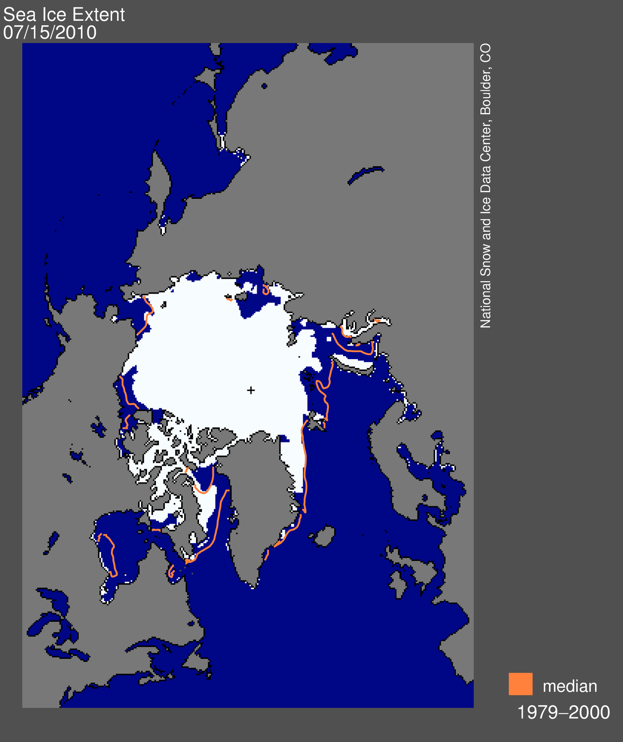
Figure 1. Daily Arctic sea ice extent on July 15 was 8.37 million square kilometers (3.23 million square miles). The orange line shows the 1979 to 2000 median extent for that day. The black cross indicates the geographic North Pole. Sea Ice Index data. About the data. —Credit: National Snow and Ice Data Center
High-resolution image

Overview of conditions

From July 1 to 15, Arctic sea ice extent declined an average of 60,500 square kilometers (23,400 square miles) per day, 22,500 square kilometers (8,690 square miles) per day slower than the 1979 to 2000 average and substantially slower than the rate of decline in May and June.

Ice extent remained lower than normal in all regions of the Arctic, with open water developing along the coasts of northwest Canada, Alaska and Siberia.

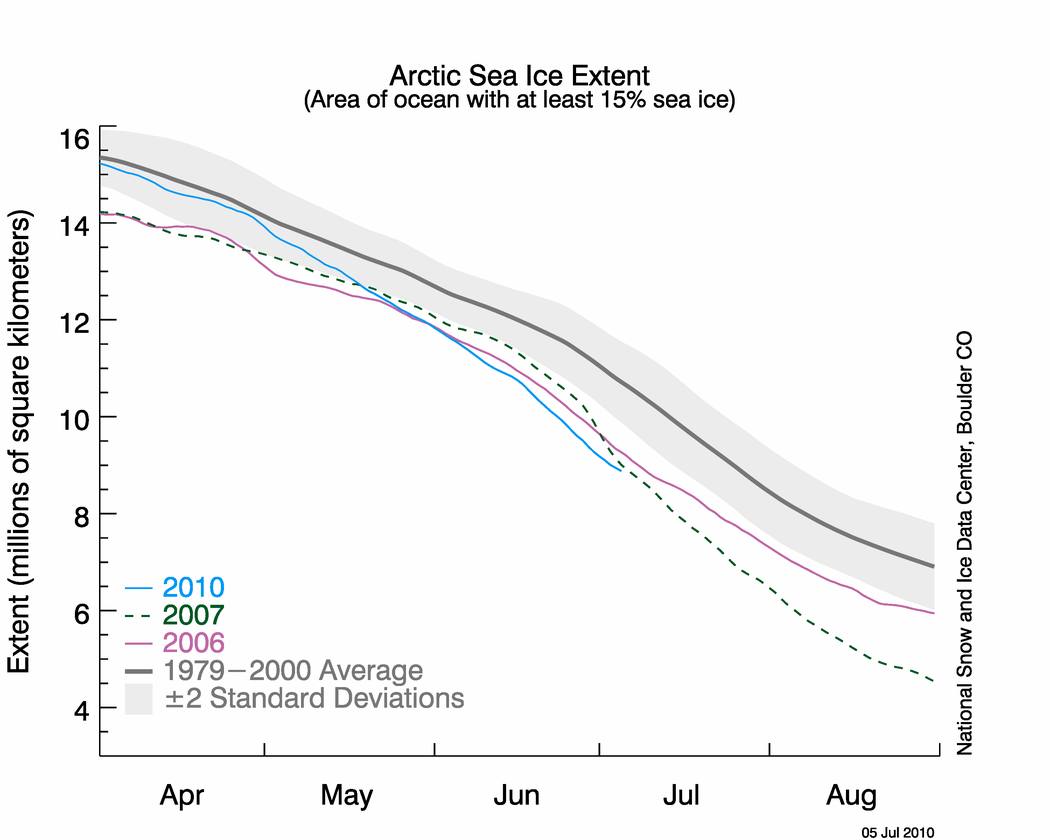
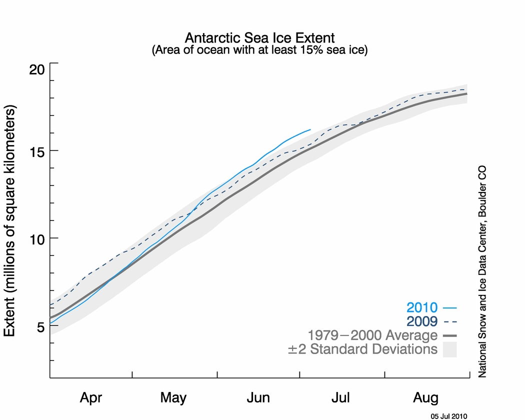
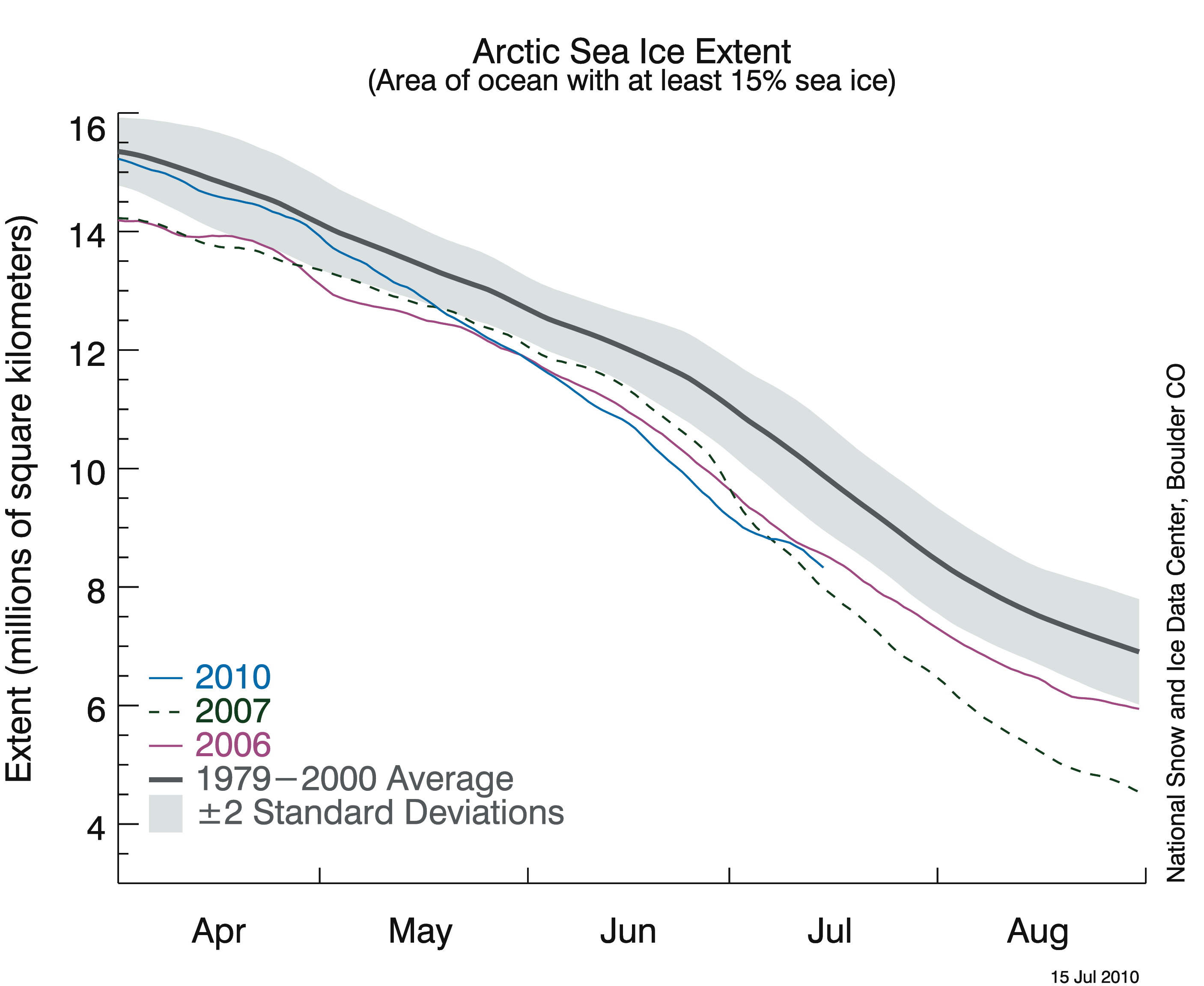
Figure 2. The graph above shows daily Arctic sea ice extent as of July 15, 2010. The solid light blue line indicates 2010; dashed green shows 2007; solid pink shows 2006, and solid gray indicates average extent from 1979 to 2000. The gray area around the average line shows the two standard deviation range of the data. Sea Ice Index data.—Credit: National Snow and Ice Data Center
High-resolution image

Conditions in context

As of July 15, total extent was 8.37 million square kilometers (3.23 million square miles), which is 1.62 million square kilometers (625,000 square miles) below the 1979 to 2000 average for the same date, but 360,000 square kilometers (139,000 square miles) above July 15, 2007, the lowest extent for that date in the satellite record.

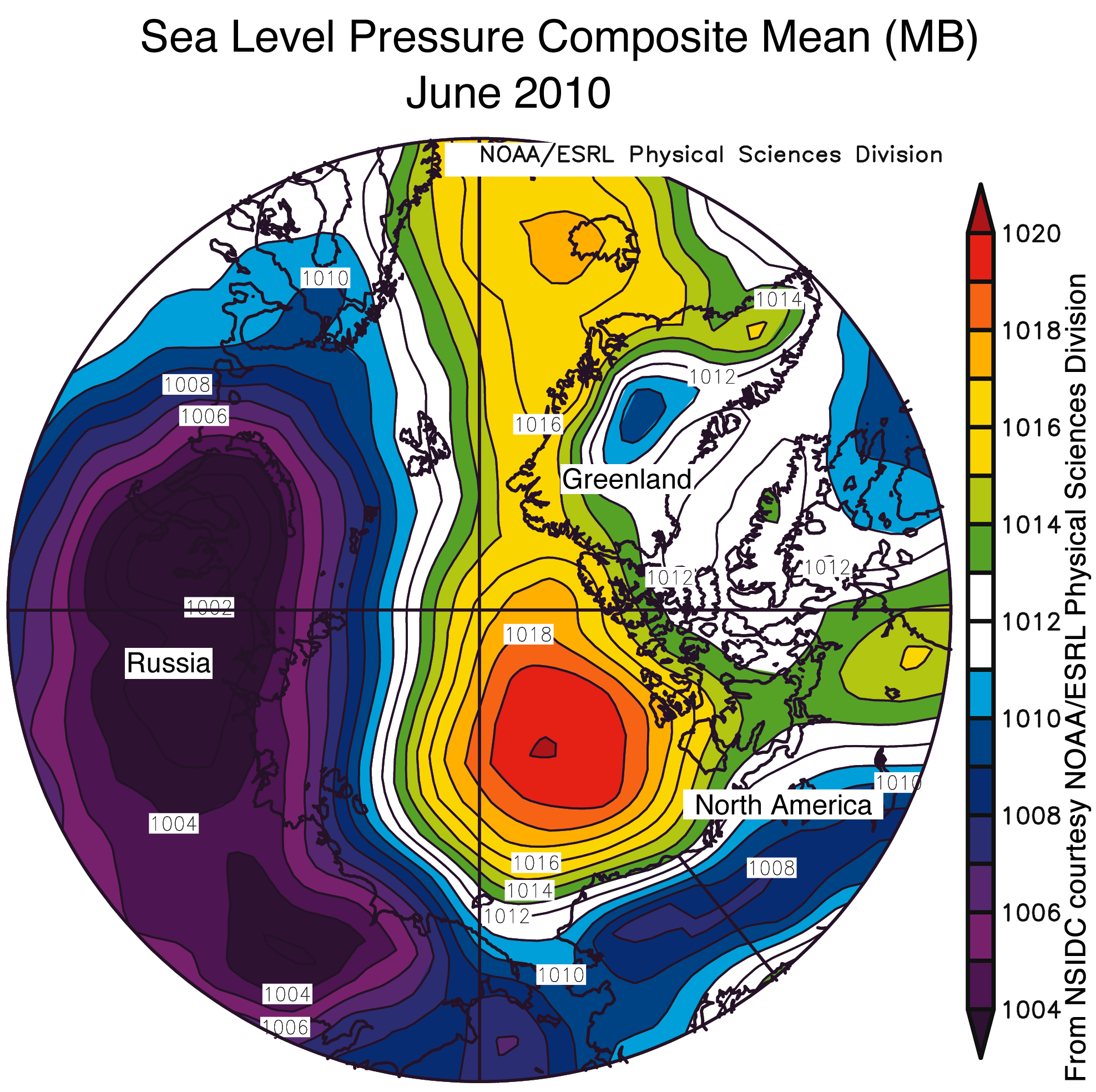
Figure 3. This map of sea level pressure for July 1 to 15, 2010 shows low pressure over the central Arctic Ocean, a pattern that brought cooler and cloudier conditions.—Credit: National Snow and Ice Data Center courtesy NOAA/ESRL Physical Sciences Division
High-resolution image

A change in circulation

Through much of May and June, high pressure dominated the Beaufort Sea with low pressure over Siberia. Winds associated with this pattern, known as the dipole anomaly, helped speed up ice loss by pushing ice away from the coast and promoting melt.

However, the dipole anomaly pattern broke down in early July. In the first half of July, cyclones (low pressure systems) generated over northern Eurasia tracked eastward along the Siberian coast and then into the central Arctic Ocean, where they tend to stall. This cyclone pattern is quite common in summer. The low-pressure cells have brought cooler and cloudier conditions over the Arctic Ocean. They have also promoted a cyclonic (anticlockwise) sea ice motion, which acts to spread the existing ice over a larger area. All of these factors likely contributed to the slower rate of ice loss over the past few weeks.

In the last few days, high pressure has started to build again in the Beaufort Sea, but whether this will continue remains to be seen.

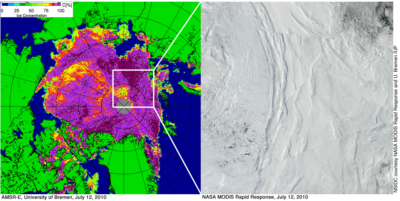
Figure 4. In mid-summer, the NASA Advanced Microwave Scanning Radiometer – Earth Observing System (AMSR-E) (left) may show areas of low ice concentration which are actually melt ponds or weather effects. Visible band images from the NASA Moderate Resolution Imaging Spectroradiometer (right) confirm areas of low-concentration sea ice in the interior pack ice. Both images are from July 12, 2010.—Credit: National Snow and Ice Data Center
High-resolution image

Areas of diffuse ice

Satellite images provided by the University of Bremen, from the NASA Advanced Microwave Scanning Radiometer – Earth Observing System (AMSR-E), show areas of low ice concentration over the central Arctic pack ice. While we normally report on the extent of area covered by at least fifteen percent sea ice, a more reliable measurement, it is also valuable to look at ice concentration values, which can reveal conditions in more detail. However, it can be difficult to interpret AMSR-E concentration data during the summer, because microwave signals associated with low ice concentration look very much like signals associated with surface melt. Weather effects can also cause false concentration signals.

By comparing AMSR-E data with data from other satellites, we can determine which areas of apparent low-concentration ice are real, and which appear to be low because of melt or atmospheric effects. Visible-band images from the NASA Moderate Resolution Imaging Spectroradiometer (MODIS) sensor show that some of the areas of apparent low ice concentration within the central pack ice are actually melt and atmospheric effects. However, the MODIS data also confirm that there are substantial areas of open water within the pack ice, such as near the North Pole and in the Beaufort Sea.

Open water in the interior pack ice is not unprecedented. Winds can push the ice apart, creating openings in the pack ice. These areas of open water may close up quickly if the wind changes, but since the dark areas of open water readily absorb solar energy, they can also lead to more extensive melt.

Further Reading

Serreze, M., and A. P. Barrett. 2007. The Summer Cyclone Maximum over the Central Arctic Ocean. Journal of Climate 21, pp. 1048-1065. doi: 10.1175/2007JCLI1810.1

Figure 1. Arctic sea ice extent for June 2010 was 10.87 million square kilometers (4.20 million square miles). The magenta line shows the 1979 to 2000 median extent for that month. The black cross indicates the geographic North Pole. Sea Ice Index data. About the data. —Credit: National Snow and Ice Data Center
High-resolution image

Overview of conditions

Arctic sea ice extent averaged 10.87 million square kilometers (4.20 million square miles) for the month of June, 1.29 million square kilometers (498,000 square miles) below the 1979 to 2000 average and 190,000 square kilometers (73,000 square miles) below the previous record low for the month of 11.06 million square kilometers (4.27 million square miles), set in 2006. In June, ice extent declined by 88,000 square kilometers (34,000 square miles) per day, more than 50% greater than the average rate of 53,000 square kilometers (20,000 square miles) per day. This rate of decline is the fastest measured for June.

During June, ice extent was below average everywhere except in the East Greenland Sea, where it was near average.

Figure 2. The graph above shows daily Arctic sea ice extent as of July 5, 2010. The solid light blue line indicates 2010; dashed green shows 2007; solid pink shows 2006, and solid gray indicates average extent from 1979 to 2000. The gray area around the average line shows the two standard deviation range of the data. Sea Ice Index data.—Credit: National Snow and Ice Data Center
High-resolution image

Conditions in context

At the end of May 2010, daily ice extent fell below the previous record low for May, recorded in 2006, and during June continued to track at record low levels. By the 30th of June, the extent was 510,000 square kilometers (197,000 square miles) below the same day in 2006.

Weather conditions, atmospheric patterns, and cloud cover over the next month will play a major role in determining whether the 2010 sea ice decline tracks at a level similar to 2007, or more like 2006. Although ice extent was greater in June 2007 than June 2006, in July 2007 the ice loss rate accelerated. That fast decline led up to the record low ice extent of September 2007.

However, it would not be surprising to see the rate of ice loss slow in coming weeks as the melt process starts to encounter thicker, second and third year ice in the central Arctic Ocean. Loss of ice has already slowed in the Beaufort and Chukchi Seas due to the tongue of thicker, older ice in the region noted in our April update.

Figure 3. Monthly June ice extent for 1979 to 2010 shows a decline of 3.5% per decade. —Credit: National Snow and Ice Data Center
High-resolution image

June 2010 compared to past years

Average ice extent for June 2010 was190,000 square kilometers (73,000 square miles) less than the previous record low for June, observed in 2006; 620,000 square kilometers (240,000 square miles) below that observed in 2007; and 1.29 million square kilometers (498,000 square miles) below the average extent for the month.

The linear rate of monthly decline for June over the 1979 to 2010 period is now 3.5% per decade. This year’s daily June rate of decline was the fastest in the satellite record; the previous record for the fastest rate of June decline was set in 1999. This rapid decline was in part driven by ice loss in Hudson Bay.

Figure 4. This map of sea level pressure for June 2010 shows a return of the Arctic dipole anomaly pattern, with unusually high pressure (yellow and orange) over the northern Beaufort Sea and unusually low pressure (purple and blue) over the Eurasian coast.—Credit: National Snow and Ice Data Center courtesy NOAA/ESRL Physical Sciences Division
High-resolution image

The Arctic dipole anomaly

The record low ice extent of September 2007 was influenced by a persistent atmospheric pressure pattern called the summer Arctic dipole anomaly (DA). The DA features unusually high pressure centered over the northern Beaufort Sea and unusually low pressure centered over the Kara Sea, along the Eurasian coast. In accord with Buys Ballot’s Law, this pattern causes winds to blow from the south along the Siberian coast, helping to push ice away from the coast and favoring strong melt. The DA pattern also promotes northerly winds in the Fram Strait region, helping to flush ice out of the Arctic Ocean into the North Atlantic. The DA pattern may also favor the import of warm ocean waters from the North Pacific that hastens ice melt.

June 2010 saw the return of the DA, but with the pressure centers shifted slightly compared to summer 2007. As a result, winds along the Siberian coastal sector are blowing more from the east rather than from the south. Whether or not the DA pattern persists through the rest of summer will bear strongly on whether a new record low in ice extent is set in September 2010.

Figure 5. This satellite image, acquired by the Moderate Resolution Imaging Spectroradiometer (MODIS) aboard the NASA Terra satellite on June 30, 2010, shows that Nares Strait was open and sea ice was flowing through it. Normally Nares Strait remains plugged by an “ice arch” through early July, but this year it was clear by May.—Credit: National Snow and Ice Data Center courtesy NASA/GSFC MODIS Rapid Response
High-resolution image

Nares Strait

Ron Kwok of the Jet Propulsion Laboratory (JPL) reports that Nares Strait, the narrow passageway between northwest Greenland and Ellesmere Island is clear of the ice “arch” that usually plugs southward transport of the old, thick ice in the Lincoln Sea. Typically the ice arch forms in winter and breaks up in early July. This year the arch formed around March 15th and lasted only 56 days, breaking up in May. In 2007 the ice arch did not form at all, allowing twice as much export through Nares Strait than the annual mean. Although the export of sea ice out of the Arctic Ocean through Nares Strait is very small in comparison to the export through Fram Strait, the Lincoln Sea contains some of the Arctic’s thickest ice. For the ice flux rates out of Nares strait, see Figure 5a.

Figure 6. The graph above shows daily Antarctic sea ice extent as of July 5, 2010. The solid light blue line indicates 2010; dashed green shows 2007, and solid gray indicates average extent from 1979 to 2000. The gray area around the average line shows the two standard deviation range of the data. Sea Ice Index data.—Credit: National Snow and Ice Data Center
High-resolution image

Meanwhile, in Antarctica

At the end of June, Southern Hemisphere mid-winter, the sea ice surrounding Antarctica was more than two standard deviations greater than normal. On June 30, Antarctic sea ice extent was15.88 million square kilometers (6.13 million square miles), compared to the 1979 to 2000 average of 14.64 million square kilometers (5.65 million square miles) for that day.

While recent studies have shown that wintertime Antarctic sea ice has a weak upward trend, and substantial variability both within a year and from year to year, the differences between Arctic and Antarctic sea ice trends are not unexpected. Climate models consistently project that the Arctic will warm more quickly than the Antarctic, largely due to the strong climate feedbacks in the Arctic. Warming is amplified by the loss of ice cover in the Arctic Ocean in areas that had been ice-covered for decades, and by the warming of Arctic lands as snow cover is lost earlier and returns later than in recent decades.

Moreover, rising levels of greenhouse gases and the loss of stratospheric ozone appear to be affecting wind patterns around Antarctica. Shifts in this circulation are referred to as the Antarctic Oscillation (AAO). As greenhouse gases have increased, and especially when ozone is lost in spring, there is a tendency for these winds to strengthen (a positive AAO index). The net effect is to push sea ice eastward, and northward, increasing the ice extent. As the current sea ice anomaly has developed, the AAO index has been strongly positive. See the NOAA AAO Index Web site. For more information about the differences between sea ice dynamics in the Arctic and Antarctic, see the NSIDC All About Sea Ice Web site.

References

Arblaster, J. M., and G. A. Meehl. 2006. Contributions of External Forcings to Southern Annular Mode Trends. Journal of Climate, 19: 2896-2905.

Hall, A., and M. Visbeck. 2002. Synchronous Variability in the Southern Hemisphere Atmosphere, Sea Ice, and Ocean Resulting from the Annular Mode. Journal of Climate, 15: 3047-3053.

Kwok, R. 2005. Variability of Nares Strait ice flux. Geophys. Res. Lett., 32, L24502, doi:10.1029/2005GL024768

Kwok, R., L. Toudal Pedersen, P. Gudmandsen, and S. S. Pang. 2010. Large sea ice outflow into the Nares Strait in 2007. Geophys. Res. Lett., 37, L03502, doi:10.1029/2009GL041872.

Thompson, W. J., and S. Solomon. 2002. Interpretation of Recent Southern Hemisphere Climate Change. Science. 296, 895-899, doi:10.1126/science.1069270

Wang, J., J. Zhang, E. Watanabe, M. Ikeda, K. Mizobata, J. E. Walsh, X. Bai, and B. Wu. 2009. Is the Dipole Anomaly a major driver to record lows in Arctic summer sea ice extent? Geophys. Res. Lett., 36, L05706, doi:10.1029/2008GL036706.